Reading: Lesson 4 - Annuities
4.4.A - Annuities
1. Annuities
- assets such as bonds provide a series of cash inflows over time, and obligations such as auto loans, student loans, and mortgages call for a series of payments. If the payments are equal and are made at fixed intervals, then we have an annuity. For example, $100 paid at the end of each of the next 3 years is a 3-year annuity.
- If payments occur at the end of each period, then we have an ordinary (or deferred) annuity. Payments on mortgages, car loans, and student loans are generally made at the ends of the periods and thus are ordinary annuities. If the payments are made at the beginning of each period, then we have an annuity due. Rental lease payments, life insurance premiums, and lottery payoffs (if you are lucky enough to win one!) are examples of annuities due. Ordinary annuities are more common in finance, so when we use the term “annuity” you may assume that the payments occur at the ends of the periods unless we state otherwise.
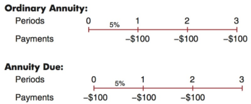
- Next we show the time lines for a $100, 3-year, 5%, ordinary annuity and for the same annuity on an annuity due basis. With the annuity due, each payment is shifted back (to the left) by 1 year. In our example, we assume that a $100 payment will be made each year, so we show the payments with minus signs.
4. As we demonstrate in the following sections, we can find an annuity’s future value, present value, the interest rate built into the contracts, how long it takes to reach a financial goal using the annuity, and, if we know all of those values, the size of the annuity payment. Keep in mind that annuities must have constant payments and a fixed number of periods. If these conditions don’t hold, then the series is not an annuity.
2. Future Value of an Ordinary Annuity
- Consider the ordinary annuity whose time line was shown previously, where you deposit $100 at the end of each year for 3 years and earn 5% per year. The figure below shows how to calculate the future value of the annuity, FVAN, using the same approaches we used for single cash flows.
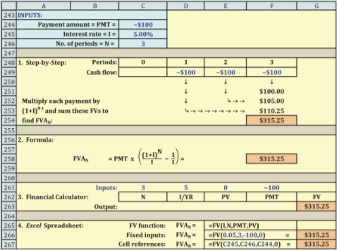
2. As shown in the step-by-step section of the above figure, we compound each payment out to Time 3, and then sum those compounded values in Cell F254 to find the annuity’s FV, FVA3 = $315.25. The first payment earns interest for two periods, the second for one period, and the third earns no interest because it is made at the end of the annuity’s life. This approach is straightforward, but if the annuity extends out for many years, it is cumbersome and time-consuming. As you can see from the time line diagram, with the step-by-step approach we apply the following equation with N = 3 and I = 5%:
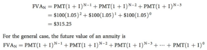
3. The Future Value of Annuity can be calculated as below:
![]()
![]()
4. Annuity problems can be solved easily using a financial calculator or a spreadsheet, most of which have the following formula built into them:
![]()
The procedure when dealing with annuities is similar to what we have done thus far for single payments, but the presence of recurring payments means that we must use the PMT key. Here’s the calculator setup for our illustrative annuity:
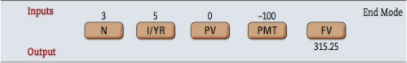
We enter PV = 0 because we start off with nothing, and we enter PMT = −100 because we will deposit this amount in the account at the end of each of the 3 years. The interest rate is 5%, and when we press the FV key we get the answer, FVA3 = 315.25. Because this is an ordinary annuity, with payments coming at the end of each year, we must set the calculator appropriately. As noted earlier, most calculators “come out of the box” set to assume that payments occur at the end of each period—that is, to deal with ordinary annuities. However, there is a key that enables us to switch between ordinary annuities and annuities due. For ordinary annuities, the designation “End Mode” or something similar is used, while for annuities due the designator is “Begin,” “Begin Mode,” “Due,” or something similar. If you make a mistake and set your calculator on Begin Mode when working with an ordinary annuity, then each payment will earn interest for 1 extra year, which will cause the compounded amounts, and thus the FVA, to be too large. The spreadsheet approach uses Excel’s FV function, =FV(I,N,PMT,PV). In our example, we have =FV(0.05,3,−100,0), and the result is again $315.25.
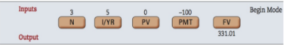
3. Future Value of an Annuity Due
- Because each payment occurs one period earlier with an annuity due, the payments will all earn interest for one additional period. Therefore, the FV of an annuity due will be greater than that of a similar ordinary annuity. If you followed the step-by-step procedure, you would see that our illustrative annuity due has a FV of $331.01 versus $315.25 for the ordinary annuity. With the formula approach, we first use the above equation, but because each payment occurs one period earlier, we multiply the result by (1 + I):
![]()
2. Thus, for the annuity due, FVAdue = $315.25(1.05) = $331.01, which is the same result as found with the step-by-step approach. With a calculator, we input the variables just as we did with the ordinary annuity, but we now set the calculator to Begin Mode to get the answer, $331.01.
3. In Excel, we still use the FV function, but we must indicate that we have an annuity due. The function is =FV(I,N,PMT,PV,Type), where “Type” indicates the type of annuity. If Type is omitted, then Excel assumes that it is 0, which indicates an ordinary annuity. For an annuity due, Type = 1. As shown in Ch04 Tool Kit.xls, the function is =FV(0.05,3,−100,0,1) = $331.01.
4. Present Value of Ordinary Annuities and Annuities Due
- The present value of any annuity, PVAN, can be found using the step-by-step, formula, calculator, or spreadsheet methods. We begin with ordinary annuities.
- we discount each payment back to Time 0, and then sum those discounted values to find the annuity’s PV, PVA3 = $272.32. This approach is straightforward, but if the annuity extends out for many years, it is cumbersome and time-consuming. The time line diagram shows that with the step-by-step approach we apply the following equation with N = 3 and I = 5%:
![]()
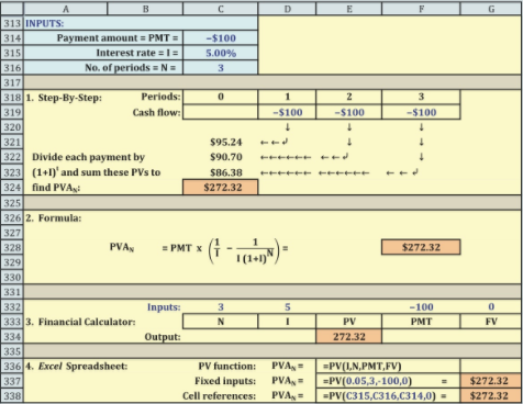
The present value of an annuity can be written as:

For our example annuity, the present value is:
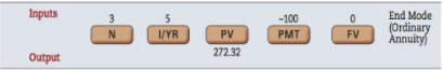
The spreadsheet solution using Excel’s built-in PV function: =PV(I,N,PMT,FV). In our example, we have =PV(0.05,3,−100,0) with a resulting value of $272.32.
5. Present Value of Annuities Due
- Because each payment for an annuity due occurs one period earlier, the payments will all be discounted for one less period. Therefore, the PV of an annuity due must be greater than that of a similar ordinary annuity. If you went through the step-by-step procedure, you would see that our example annuity due has a PV of $285.94 versus $272.32 for the ordinary annuity. With the formula approach, we first use the below equation to find the value of the ordinary annuity and then, because each payment now occurs one period earlier, we multiply the equation result by (1 + I):

With a financial calculator, the inputs are the same as for an ordinary annuity, except you must set the calculator to Begin Mode:
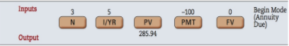
2. In Excel, we again use the PV function, but now we must indicate that we have an annuity due. The function is now =PV(I,N,PMT,FV,Type), where “Type” is the type of annuity. If Type is omitted then Excel assumes that it is 0, which indicates an ordinary annuity; for an annuity due, Type = 1 the function for this example is =PV(0.05,3,−100,0,1) = $285.94.
Last modified: Tuesday, August 14, 2018, 8:41 AM