Reading: Lesson 4 - Forecasting When the Ratios Change
10.4.A - Forecasting When the Ratios Change
1. Forecasting When the Ratios Change
- The versions of the percent of sales forecasting model and the AFN method assumed that the forecasted items could be estimated as a percent of sales. This implies that each of the accounts for assets, spontaneous liabilities, and operating costs is proportional to sales. In graph form, this implies the type of relationship shown in Panel a of the Figure below, a relationship whose graph (1) is linear and (2) passes through the origin. Under those conditions, if the company’s sales increase from $200 million to $400 million, or by 100%, then inventory will also increase by 100%, from $100 million to $200 million. The assumption of constant ratios and identical growth rates is appropriate at times, but there are times when it is incorrect.

There are economies of scale in the use of many kinds of assets, and when economies of scale occur, the ratios are likely to change over time as the size of the firm increases. For example, retailers often need to maintain base stocks of different inventory items even if current sales are quite low. As sales expand, inventories may then grow less rapidly than sales, so the ratio of inventory to sales (I/S) declines. This situation is depicted in Panel b of the Figure above. Here we see that the inventory/sales ratio is 1.5 (or 150%) when sales are $200 million but declines to 1.0 when sales climb to $400 million.
The relationship in Panel b is linear, but nonlinear relationships often exist. Indeed, if the firm uses one popular model for establishing inventory levels (the Economic Ordering Quantity, or EOQ, model), its inventories will rise with the square root of sales. This situation is shown in Panel c of the Figure above, which shows a curved line whose slope decreases at higher sales levels. In this situation, very large increases in sales would require very little additional inventory. To incorporate this type of nonlinearity in Excel, for example, you could forecast inventory as a function of the square root of sales: Inventory = m(Sales0.5).
In many industries, technological considerations dictate that if a firm is to be competitive, it must add fixed assets in large, discrete units; such assets are often referred to as lumpy assets. In the paper industry, for example, there are strong economies of scale in basic paper mill equipment, so when a paper company expands capacity, it must do so in large, lumpy increments. This type of situation is depicted in Panel d of Figure 12-8. Here we assume that the minimum economically efficient plant has a cost of $75 million, and that such a plant can produce enough output to reach a sales level of $100 million. If the firm is to be competitive, it simply must have at least $75 million of fixed assets.
Lumpy assets have a major effect on the ratio of fixed assets to sales (FA/S) at different sales levels and, consequently, on financial requirements. At Point A in Panel d, which represents a sales level of $50 million, the fixed assets are $75 million and so the ratio FA/S = $75/$50 = 1.5. Sales can expand by $50 million, out to $100 million, with no additions to fixed assets. At that point, represented by Point B, the ratio FA/S = $75/$100 = 0.75. However, because the firm is operating at capacity (sales of $100 million), even a small increase in sales would require a doubling of plant capacity, so a small projected sales increase would bring with it a large financial requirement.
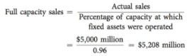
If assets are lumpy and a firm makes a major purchase, the firm will have excess capacity, which means that sales can grow before the firm must add capacity. The level of full capacity sales is

For example, consider MicroDrive and use the data from its financial statements, but now assume that excess capacity exists in fixed assets. Specifically, assume that fixed assets in 2013 were being utilized to only 96% of capacity. If fixed assets had been used to full capacity, then 2013 sales could have been as high as $3,125 million versus the $3,000 million in actual sales:
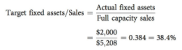
The target fixed assets/sales ratio can be defined in terms of the full capacity sales:

MicroDrive’s target fixed assets/sales ratio should be 38.4% rather than 40%:
The required level of fixed assets depends upon this target fixed assets/sales ratio:

Therefore, if MicroDrive’s sales increase to $3,300 million, its fixed assets would have to increase to $1,056 million:

We previously forecasted that MicroDrive would need to increase fixed assets at the same rate as sales, or by 10%. That meant an increase of $200 million, from $2,000 million to $2,200 million under the old assumption of no excess capacity. Under the new assumption of excess capacity, the actual required increase in fixed assets is only from $2,000 million to $2,112 million, which is an increase of $112 million. Thus, the capacity- adjusted forecast is less than the earlier forecast: $200 − $112 = $88 million. With a smaller fixed asset requirement, the projected AFN would decline from an estimated $118 million to $118 − $88 = $30 million.
Note also that when excess capacity exists, sales can grow to the capacity sales as calculated above with no increase in fixed assets, but sales beyond that level would require additions of fixed assets as in our example. The same situation could occur with respect to inventories, and the required additions would be determined in exactly the same manner as for fixed assets. Theoretically, the same situation could occur with other types of assets, but as a practical matter excess capacity normally exists only with respect to fixed assets and inventories.
Last modified: Tuesday, August 14, 2018, 8:52 AM