Reading: Lesson 2 - After-Tax Cost of Debt
8.2.A - After-Tax Cost of Debt
1. The Before-Tax Cost of Short-Term Debt
- Short-term debt should be included in the capital structure only if it is a permanent source of financing in the sense that the company plans to continually repay and refinance the short-term debt. This is the case for MicroDrive, whose bankers charge 10% on notes payable. Therefore, MicroDrive’s short-term lenders have a required return of rstd = 10%, which is MicroDrive’s before-tax cost of short-term debt.
2. The Before-Tax Cost of Long-Term Debt
- For long-term debt, estimating rd is conceptually straightforward, but some problems arise in practice. Companies use both fixed- and floating-rate debt, both straight and convertible debt, both long- and short-term debt, as well as debt with and without sinking funds. Each type of debt may have a somewhat different cost.
- It is unlikely that the financial manager will know at the beginning of a planning period the exact types and amounts of debt that will be used during the period. The type or types used will depend on the specific assets to be financed and on capital market conditions as they develop over time. Even so, the financial manager does know what types of debt are typical for his firm. For example, MicroDrive typically issues 15-year bonds to raise long-term debt used to help finance its capital budgeting projects. Because the WACC is used primarily in capital budgeting, MicroDrive’s treasurer uses the cost of 15-year bonds in her WACC estimate.
- Assume that it is January 2014 and that MicroDrive’s treasurer is estimating the WACC for the coming year. How should she calculate the component cost of debt? Most financial managers begin by discussing current and prospective interest rates with their investment bankers. Assume MicroDrive’s bankers believe that a new, 15-year, noncallable, straight bond issue would require a 9% coupon rate with semiannual payments. It can be offered to the public at its $1,000 par value. Therefore, their estimate of rd is 9%.
- Note that 9% is the cost of new, or marginal, debt, and it will probably not be the same as the average rate on MicroDrive’s previously issued debt, which is called the historical, or embedded, rate. The embedded cost is important for some decisions but not for others. For example, the average cost of all the capital raised in the past and still outstanding is used by regulators when they determine the rate of return that a public utility should be allowed to earn. However, in financial management the WACC is used primarily to make investment decisions, and these decisions hinge on projects’ expected future returns versus the cost of the new, or marginal, capital that will be used to finance those projects. Thus, for our purposes, the relevant cost is the marginal cost of new debt to be raised during the planning period.
- MicroDrive has issued debt in the past and the bonds are publicly traded. The financial staff can use the market price of the bonds to find the yield to maturity (or yield to call, if the bonds sell at a premium and are likely to be called). This yield is the rate of return that current bondholders expect to receive, and it is also a good estimate of rd, the rate of return that new bondholders will require.
- MicroDrive’s outstanding bonds were recently issued and have a 9% coupon, paid semiannually. The bonds mature in 15 years and have a par value of $1,000. These bonds are trading at $1,000. We can find the yield to maturity by using a financial calculator with these inputs: N = 30, PV = −1000, PMT = 45, and FV = 1000. Solving for the rate, we find I/YR = 4.5%. This is a semiannual periodic rate, so the nominal annual rate is 9.0%. This is consistent with the investment bankers’ estimated rate, so 9% is a reasonable estimate for rd.
- MicroDrive’s outstanding bonds are trading at par, so the yield is equal to the coupon rate. But consider a hypothetical example for which the market price isn’t par but instead is $923.14. We can find the yield to maturity by using a financial calculator with these inputs: N = 30, PV = −923.14, PMT = 45, and FV = 1000. Solving for the rate, we find I/YR = 5%, which implies a hypothetical nominal annual rate of 10%. As this hypothetical example illustrates, it is not necessary for the bond to trade at par in order to estimate the cost of debt.
- Be alert to situations in which there is a significant probability that the company will default on its debt. In such a case, the yield to maturity (whether calculated from market prices of an outstanding bond or taken as the coupon rate on a newly issued bond) overstates the investor’s expected return and hence the company’s expected cost. For example, let’s reconsider MicroDrive’s 15-year semiannual bonds that can be issued at par if the coupon rate is 9%. As shown previously, the nominal annual yield to maturity is 9%. But suppose investors believe there is a significant chance that MicroDrive will default. To keep the example simple, suppose investors believe that the bonds will default in 14 years and that the recovery rate on the par value will be 70%. Here are the new inputs: N = 2(14) = 28, PV = −1000, PMT = 45, and FV = 0.70(1000) = 700. Solving for the rate, we find I/YR = 3.9%, implying an annual expected return of 7.8%. This is an extremely simple example, but it illustrates that the expected return on a bond is less than the yield to maturity as it is normally calculated. For bonds with a relatively low expected default rate, we recommend using the yield to maturity.
3. The After-Tax Cost of Debt
- The required return to debtholders, rd, is not equal to the company’s cost of debt because interest payments are deductible, which means the government in effect pays part of the total cost. As a result, the weighted average cost of capital is calculated using the after-tax cost of debt, rd(1 − T), which is the interest rate on debt, rd, less the tax savings that result because interest is deductible. Here T is the firm’s marginal tax rate.
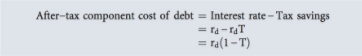
If we assume that MicroDrive’s marginal federal-plus-state tax rate is 40%, then its after-tax cost of debt is 5.4%:
For MicroDrive’s short-term debt, the after-tax cost is 6%: rstd(1 − T) = 10%(1.0 − 0.4) = 6%.
4. Flotation Costs and the Cost of Debt
- Most debt offerings have very low flotation costs, especially for privately placed debt. Because flotation costs are usually low, most analysts ignore them when estimating the after-tax cost of debt. However, the following example illustrates the procedure for incorporating flotation costs as well as their impact on the after-tax cost of debt.
- Suppose MicroDrive can issue 30-year debt with an annual coupon rate of 9%, with coupons paid semiannually. The flotation costs, F, are equal to 1% of the value of the issue. Instead of finding the pre-tax yield based upon pre-tax cash flows and then adjusting it to reflect taxes, as we did before, we can find the after-tax, flotation-adjusted cost by using this formula:

Here M is the bond’s maturity (or par) value, F is the percentage flotation cost (i.e., the percentage of proceeds paid to the investment bankers), N is the number of payments, T is the firm’s tax rate, INT is the dollars of interest per period, and rd(1 − T) is the after-tax cost of debt adjusted for flotation costs. With a financial calculator, enter N = 60, PV = −1000(1 − 0.01) = −990, PMT = 45(1 − 0.40) = 27, and FV = 1000. Solving for I/YR, we find I/YR = rd(1 − T) = 2.73%, which is the semiannual after-tax component cost of debt. The nominal after-tax cost of debt is 5.46%. Note that this is quite close to the original 5.40% after-tax cost, so in this instance adjusting for flotation costs doesn’t make much difference.
However, the flotation adjustment would be higher if F were larger or if the bond’s life were shorter. For example, if F were 10% rather than 1%, then the nominal annual flotation- adjusted rd(1 − T) would be 6.13%. With N at 1 year rather than 30 years and F still equal to 1%, the nominal annual rd(1 − T) = 6.45%. Finally, if F = 10% and N = 1, then the nominal annual rd(1 − T) = 16.67%. In all of these cases, the effect of flotation costs would be too large to ignore.
As an alternative to adjusting the cost of debt for flotation costs, in some situations it makes sense to instead adjust the project’s cash flows. For example, project financing is a special situation in which a large project, such as an oil refinery, is financed with debt plus other securities that have a specific claim on the project’s cash flows. This is different from the usual debt offering, in which the debt has a claim on all of the corporation’s cash flows. Because project financing is funded by securities with claims tied to a particular project, the flotation costs can be included with the project’s other cash flows when evaluating the project’s value. However, project financing is relatively rare, so when we incorporate the impact of flotation costs, we usually do so by adjusting the component cost of the new debt.
Modifié le: mardi 14 août 2018, 08:50