Reading: Lesson 2 - From Financial Crisis to Recession
1. From Housing to the Aggregate Economy
The aggregate expenditure model takes as its starting point the fact that gross domestic product (GDP) measures both total spending and total production. When planned and actual spending are in balance,
real GDP = planned spending= autonomous spending + marginal propensity to spend × real GDPAutonomous spending is the intercept of the planned spending line. It is the amount of spending that there would be in the economy if income were zero. The equilibrium level of real GDP is as follows:
The framework tells us that a reduction in autonomous spending leads to a decrease in real GDP.
Just as in the Great Depression, the two leading candidates for the decrease in autonomous spending are consumption and investment. Specifically, the crisis in the housing market had two significant implications for the rest of the economy. First, the decrease in housing prices starting in 2008 reduced the wealth of many households. Because households were poorer, they reduced their consumption. Second, the disruptions in the financial system made it difficult for firms to obtain financing, which meant that there was less investment. The aggregate expenditure model teaches us that these reductions in consumption and investment can lead to a reduction in real GDP.
Reductions in autonomous spending are magnified through the circular flow of income. As spending decreases, income decreases, leading to further reductions in spending. This is the multiplier process; it shows up as the term 1/(1 − marginal propensity to spend), which multiplies autonomous spending in the expression for real GDP.
2. Stabilization Policy
We have already observed that, in contrast to the Great Depression, policymakers in the crisis of 2008 took several actions to try to address the economic problems. In addition to the measures aimed specifically at dealing with problems in the financial markets, policymakers turned to monetary and fiscal policy in an attempt to counteract the economic downturn.
To begin our discussion of this stabilization policy, it is useful to start with a summary of the state of the economy in the 2006–10 period. By so doing, we are making life somewhat easier for us than it was for policymakers because they did not know in early 2009 what would happen in the aggregate economy during that year. The annual growth rates of the main macroeconomic variables during the crisis are highlighted in the Table below "State of the Economy: Growth Rates from 2006 to 2010". All variables are in percentage terms.
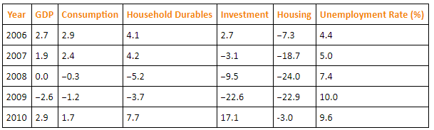
One of the priorities of the Obama administration after taking office in January 2009 was to formulate a stimulus package to deal with the looming recession. As is clear from the Table above "State of the Economy: Growth Rates from 2006 to 2010", growth in the economy was near zero for the preceding year, and the unemployment rate was much higher than it had been in the previous two years. Although the financial rescue plans of the George W. Bush administration may have stemmed the financial crisis, the aggregate economy was now limping along at best.
The American Recovery and Reinvestment Act of 2009 (ARRA) was signed into law on February 17, 2009. The stimulus package contained approximately $800 billion in spending increases and tax cuts. These numbers are approximate for a couple of reasons: (1) parts of the package depend on the state of the economy in the future, so the exact outlays are not determined in the legislation, and (2) the disbursements were not all within a single year, so the timing of the outlays and thus their discounted present value could not be precisely known at the time of passage.
The package contained a mixture of spending increases and tax cuts. According to a Congressional Budget Office (CBO) study (http://www.cbo.gov/ftpdocs/106xx/doc10682/Frontmatter.2.2.shtml) from November 2009, federal government purchases of goods and services were to increase by about $90 billion over the 2009–19 period. Transfer payments to households were set to increase by about $100 billion, and transfers to state and local governments were to increase by nearly $260 billion. This last category of outlays was quite visible, taking the form of road projects and other construction in towns across the United States. Interestingly, the federal government was investing in infrastructure, thus building up the public component of the capital stock.
In the same publication, the CBO provided a summary of ARRA’s macroeconomic effects in November 2009. At that point, due to ARRA, the CBO estimated that federal government outlays (not only spending on goods and services) had increased by about $100 billion, and tax collections were lower by about $90 billion. So clearly some but not the entire stimulus went into the US economy within seven months of ARRA’s passage. The CBO also produced its own assessment of the effects of ARRA through September 2009. To do so, it had to use an economic model to calculate the effects of the increases in outlays and reductions in taxes.
According to the CBO, ARRA meant that real GDP in the United States was between 1.2 percent and 3.2 percent higher than it would otherwise have been, whereas the unemployment rate was between 0.3 and 0.9 percentage points lower. These numbers were obtained by attaching a multiplier to each component of the stimulus package and calculating the change in real GDP from that component. For example, the CBO estimated that the multiplier associated with federal government purchases of goods and services was between 1 and 2.5. The effect of this federal spending on real GDP is simply the product of the spending of the federal government funded under ARRA times the multiplier. The CBO did this calculation for each component of the stimulus package and then added up the effects on real GDP. The range of the effects reflects the range for each multiplier used in their analysis. The CBO also calculated that 640,000 jobs were either created or retained due to ARRA. This calculation underlies their estimate of how much ARRA reduced the unemployment rate in the United States.
Some economists have disputed the effects of ARRA on economic activity, however. John Taylor, a Stanford University economist, argued that the short-term nature of the tax cuts meant that most households simply saved the tax cut, as the theory of consumption smoothing predicts. This argument was supported by evidence of increasing saving rates by households in the United States during the period of the tax cuts.Testimony reproduced in John B. Taylor, “The 2009 Stimulus Package: Two Years Later,” Hoover Institution, February 16, 2011, accessed September 20, 2011, http://media.hoover.org/sites/default/files/documents/2009-Stimulus-two-years-later.pdf.
During 2010 and 2011, there were some calls for further stimulus. The unemployment rate in the United States remained high despite the stimulus; it was 9.5 percent in July 2010. The Bureau of Labor Statistics (http://www.bls.gov/news.release/empsit.b.htm) tells us that while job creation had been brisk in May 2010 at 432,000 jobs, the total job destruction in June and July 2010 was 350,000. Further, real GDP growth was only 2.4 percent in the second quarter of 2010, down from 3.7 percent in the first quarter. Together this news put more pressure on policymakers to conduct further attempts at stabilization policy.
But at the same time, policymakers became increasingly concerned about the long-run fiscal health of the government. In effect, they began to worry about the government budget constraint, which we explained in Unit 11 "Balancing the Budget". The attention of policymakers moved away from stimulus and toward “fiscal consolidation.” This culminated in a political battle in the summer of 2011 over an increase in the debt ceiling, a limit on the amount of US debt outstanding. Ultimately an agreement was reached to allow an increase in the ceiling, but this agreement was combined with a reduction in government spending of nearly $900 billion over the coming 10 years and an agreement to seek further cuts in spending amounting to another $1.5 trillion.The bill passed by the House of Representatives is contained here: “Text of Budget Control Act Amendment,” House of Representatives Committee on Rules, accessed September 20, 2011, http://rules.house.gov/Media/file/PDF_112_1/Floor_Text/DEBT_016_xml.pdf. This agreement was not enough to avert a downgrade of US debt from AAA to AA+ by Standard and Poors.The decision to downgrade the debt is discussed at “Research Update: United States of America Long-Term Rating Lowered to ‘AA+’ on Political Risks and Rising Debt Burden; Outlook Negative,” Standard & Poor’s, August 5, 2011, accessed September 20, 2011, http://www.standardandpoors.com/servlet/BlobServer?blobheadername3 =MDT-Type&blobcol=urldata&blobtable=MungoBlobs&blobheadervalue 2=inline%3B+filename%3DUS_Downgraded_AA%2B.pdf&blobheadername2=Content-Dis position&blobheadervalue1=application%2Fpdf&blobkey=id&blob headername1=content-type&blobwhere=1243942957443&blobh eadervalue3=UTF-8.
3. Monetary Policy
- The current state of monetary policy is well summarized in the Federal Open Market Committee (FOMC) statement of August 10, 2010. Here is an excerpt:“Press Release,” Federal Open Market Committee, August 10, 2010, accessed July 26, 2011, http://www.federalreserve.gov/newsevents/press/monetary/20100810a.htm.
- We can make several observations about this FOMC statement. First, the FOMC shared the general perception that the recovery is not very robust and is showing signs of slowing. Their response was to maintain the targeted federal funds rate at between 0 and 0.25 percent. The FOMC put the targeted rate into this range in December 2008; in August 2011 the Fed indicated that it would keep rates low for at least another two years.You can find the FOMC statements and minutes of the meetings from December 2008 onward at “Meeting Calendars, Statements, and Minutes (2006–2012),” Federal Reserve, accessed July 26, 2011, http://www.federalreserve.gov/monetarypolicy/fomccalendars.htm.
- Second, the FOMC talks about “reinvesting principal payments from agency debt and agency mortgage-backed securities….” This somewhat complicated phrase refers to the fact that the Fed purchased various assets in the attempt to keep financial markets working during the financial crisis.Those programs are summarized at “Credit and Liquidity Programs and the Balance Sheet,” Federal Reserve, accessed July 26, 2011, http://www.federalreserve.gov/monetarypolicy/bst_crisisresponse.htm. As reported by the Fed, “[s]ince the beginning of the financial market turmoil in August 2007, the Federal Reserve’s balance sheet has grown in size and has changed in composition. Total assets of the Federal Reserve have increased significantly from $869 billion on August 8, 2007, to well over $2 trillion.”The Fed maintains an interactive web site that displays and explains its balance sheet items. “Credit and Liquidity Programs and the Balance Sheet,” Federal Reserve, accessed July 26, 2011, http://www.federalreserve.gov/monetarypolicy/bst_recenttrends.htm. Observers are waiting for the Fed to reduce its holdings of these assets. The policy statement indicated that the Fed was not yet ready to take those steps.
- The final point concerns the position of Thomas Hoenig, the president of the Federal Reserve Bank of Kansas City. Over the year, he took the view that monetary policy was too lax. As the economy recovered, there was, he believed, no longer any need to keep interest rates at such low levels. One of the implicit concerns here is that periods of low interest rates have tended to promote bubbles in assets, such as housing. The FOMC had to weigh this concern against the view that, with a slow economic recovery and no signs of inflation, expansionary monetary policy was still warranted. When the FOMC took the unusual decision to commit to low interest rates for two years, three members of the committee dissented from the decision.
Last modified: Tuesday, May 28, 2019, 1:23 PM