Reading: Lesson 2 - Individual Demand
1. Individual Demand for a Good
- Now that we have a framework for thinking about your choices, we can now explain one of the most fundamental economic ideas: demand. Here we focus on the demand of a single individual. We use two different ways of thinking about your demand for a good or a service. One approach builds on the idea of the budget set. The other focuses on how much you would be willing to pay for a good or service. In combination, they give us a detailed understanding of how economic decisions are made.
As you visit stores at different times, you undoubtedly notice that the prices of goods and services change. At the same time, your income may also change from one month to the next. So if we were to look at your budget set monthly, we would typically find it changing from one month to the next. We would then expect that you would choose different combinations of goods and services from one month to the next.
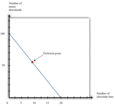
To keep things simple, suppose we are still in a world of two goods—downloads and chocolate bars—and that you do no saving. We will describe your demand for chocolate bars. (If you like, you can think of downloads as representing all the other goods and services you consume.) Given prices and your income, you pick the best point on the budget line. Look again at the “preferred” point in the Figure below "Choosing a Preferred Point on the Budget Line". One way to interpret this point is that it tells us how many chocolate bars you will buy, given your income and given the price of a chocolate bar and other goods. Using this as a reference point, we now ask how your choice will change as income changes and then as the price of a chocolate bar changes.
2. Changes in Income
- Imagine that your income increases. The Figure below "An Increase in Income" shows what happens to the budget line. Higher income means that you can afford to buy more chocolate bars and more downloads, so the budget line shifts outward. The slope of the budget line is unchanged because there is no change in the price of a chocolate bar relative to downloads.
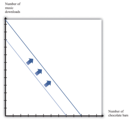
Note: An increase in income shifts the budget line outward.
What happens to your consumption of chocolate bars? There are two possibilities (the Figure below "The Consequences of an Increase in Income"): the increase in income leads you to consume either more chocolate bars or fewer chocolate bars. Both are plausible, and either is possible. (Of course, you might also choose exactly the same amount as before.) We might think that the more normal case is that higher income would lead to higher chocolate bar consumption. If a good has a property that you will consume more of it when you have higher income, we call it a normal good.
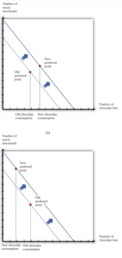
Note: In response to an increase in income, two things are possible: the consumption of chocolate bars may increase (a) or decrease (b).
Under some circumstances, higher income leads to lower consumption. For example, suppose you are surviving in college on a diet consisting of mostly instant noodles. When you graduate college and have higher income, you can afford better things to eat, so you will probably consume a smaller quantity of instant noodles. Economists call such products inferior goods. If a particular product exists in several qualities (cheap versus expensive cuts of meat, for example), we often find that the low-quality version is an inferior good. A good might be normal for one consumer and inferior for another. More precisely, therefore, we say that a good is inferior if, on average, higher income leads to lower consumption.
Economists make a further distinction among different kinds of normal goods. If you spend a larger fraction of your income on a particular good as your income increases, then we say that the good is a luxury good. Another way of saying this is that for a luxury good, the percentage increase in consumption is bigger than the percentage increase in income.
We can also define these ideas in terms of the income elasticity of demand, which is a measure of how sensitive demand is to changes in income. For an inferior good, the income elasticity of demand is negative: higher income leads to lower consumption. For a normal good, the income elasticity of demand is positive. And for a luxury good, the income elasticity of demand is greater than one.
The distinctions among these different kinds of goods are crucial for managers of firms. To predict sales, managers need to know whether the products they are selling are normal, inferior, or luxury goods. Firms that sell inferior goods tend to do well when the economy as a whole is doing poorly and vice versa. By contrast, firms selling luxury goods will do particularly poorly when the economy as a whole is performing poorly.
3. Changes in Price
- Now we look at what happens if there is a change in the price of a chocolate bar. Suppose the price decreases. First, let us analyze what this means in terms of our picture. Remember that the intercepts of the budget line tell you how much you can have of one good if you consume none of the other. If you consume no chocolate bars, then a decrease in the price of a chocolate bar has no effect on your consumption. You can consume exactly the same number of downloads as before. The intercept on the vertical axis therefore does not move. However, a decrease in the price of a chocolate bar means that, if you consume only chocolate bars, then you can have more than before. The intercept on the horizontal axis moves outward.
- The Figure below "A Decrease in the Price of a Chocolate Bar" illustrates a decrease in the price of a chocolate bar. The new budget line lies outside the old budget line. Any bundle you could have bought at the old prices is still affordable now, and you can also get more. A decrease in the price of a chocolate bar, in other words, makes you better off. In addition, the slope of the budget line changes: it is flatter than before. The slope of the budget line reflects the way in which the market allows you to trade chocolate bars for other products. If you choose to consume fewer downloads, the reduction in the price of a chocolate bar means that you get relatively more chocolate bars in exchange.
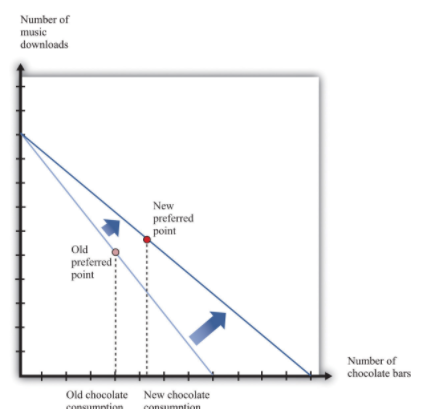
Note: A decrease in the price of a chocolate bar causes the budget line to rotate. The result is an increase in the quantity of chocolate bars consumed.
The Figure above "A Decrease in the Price of a Chocolate Bar" also shows a new consumption point. In response to the decrease in the price of a chocolate bar, we see an increase in the consumption of chocolate bars. The idea that people almost always consume more of a good when its price decreases is one of the fundamental ideas of economics. Indeed, it is sometimes called the law of demand. It is certainly intuitive that lower prices lead people to consume more. There are two reasons why we expect to see this result.
First, if a good (for example, chocolate bars) decreases in price, it becomes cheaper relative to other goods. Its opportunity cost—that is, the amount of other goods you must give up to get a chocolate bar—has decreased. The lower opportunity cost means that there is a substitution effect away from other goods and toward chocolate bars. Second, a decrease in the price of a chocolate bar also means that you can afford more of everything, including chocolate bars. Provided chocolate bars are a normal good, this income effect will also lead you to want to consume more chocolate bars. If chocolate bars are inferior goods, the income effect leads you to want to consume fewer chocolate bars.
In the Figure above "A Decrease in the Price of a Chocolate Bar", the substitution effect is reflected by the fact that the budget line changes slope. The flatter budget line tells us that the opportunity cost of chocolate bars in terms of downloads has decreased. The income effect shows up in the fact that the new budget set includes the old budget set. You can consume your previous bundle of goods and still have some income left over to buy more.
Based on the idea of the law of demand, we can construct your individual demand curve for chocolate bars. We do so by drawing the budget set for each different price of a chocolate bar, seeing how much you buy, and then plotting this data. For example, we might find that your purchases of chocolate bars look like those in the Table below "Demand for Chocolate Bars". If we plot these points on a graph and then “fill in the gaps,” we get a diagram like the second Figure below "The Demand Curve". This is your demand curve for chocolate bars. It tells how many chocolate bars you would purchase at any given price. The law of demand means that we expect this curve to slope downward. If the price increases, you consume less. If the price decreases, you consume more.
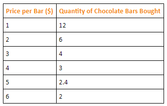
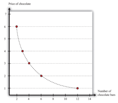
Note: The Table above "Demand for Chocolate Bars" contains an example of some observations on demand. At different prices from $1 to $6, we see the number of chocolate bars purchased. If we fill in the gaps, we obtain a demand curve.
We must be careful to distinguish between movements along the demand curve and shifts in the demand curve. Suppose there is a change in the price of a chocolate bar. Then, as we explained earlier, the budget line shifts, and the quantity demanded of both chocolate bars and downloads will change. This appears in the Figure above "The Demand Curve" as a movement along the demand curve. For example, if the price of a chocolate bar decreases from $4 to $3, then, as in the Table above "Demand for Chocolate Bars", the quantity demanded increases from three bars to four bars. The demand curve does not change; we simply move from one point on the line to another.
If a change in anything other than the price of a chocolate bar causes you to change your consumption of chocolate bars, then there is a shift in the demand curve. For example, suppose you get a pay raise at your job, so you have more income. As long as chocolate bars are a normal good, this increase in income will cause your demand curve for chocolate bars to shift outward. This means that, at any given price, you will buy more of the good when income increases. In the case of an inferior good, an increase in income will cause the demand curve to shift inward. You will buy less of the good when income increases. We illustrate these two cases in the Figure below "Shifts in the Demand Curve: Normal and Inferior Goods".
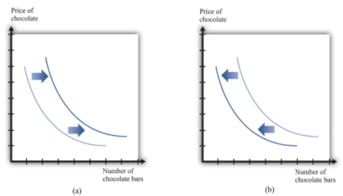
Note: (a) If income increases and chocolate bars are a normal good, then the individual demand curve will shift to the right. At every price, a greater quantity of chocolate bars is demanded. (b) If income increases and chocolate bars are inferior goods, then the individual demand curve will shift to the left. In the event of a decrease in income, the two cases are reversed.
4. Exceptions to the Law of Demand
The law of demand is highly intuitive and is supported by lots of research for all sorts of different goods and services. We can take it as a reliable fact that in almost all circumstances, the demand curve will indeed slope downward. Yet we might still wonder if there are any exceptions, any cases in which the demand curve slopes upward. There are indeed a few such exceptions.
- Giffen goods. We explained that the law of demand comes from both a substitution effect and—for normal goods—an income effect. But for inferior goods, the income effect acts in the opposite direction to the substitution effect: a decrease in price makes people better off, which is an incentive to consume less of the good. Theoretically, it is possible for this income effect to be stronger than the substitution effect. Although conceivable, Giffen goods are extremely rare; indeed, economists are unsure if they actually exist outside of textbooks. For the income effect to overwhelm the substitution effect, the good in question must form a very large part of the overall consumption bundle. This might arise in extremely poor economies where people spend a large part of their income on a staple food, as was found in a recent experiment conducted in rural China.See Robert Jensen and Nolan Miller, “Giffen Behavior: Theory and Evidence” (Harvard University, John F. Kennedy School of Government Working Paper RWP 07-030, July 2007). The researchers gave families subsidies to buy rice, making it cheaper, and found that consumption of rice did indeed decrease.
- Status goods. Some luxury products are purchased mainly for their status appeal—for example, Rolls-Royce automobiles, Louis Vuitton handbags, and Gucci shoes. The high prices of these goods contribute to their exclusivity. Price is an attribute of a good, so a higher price can make a good seem more, not less, attractive. Again, it is theoretically possible that this could lead the demand curve to slope upward, at least for some range of prices. Although high prices increase the appeal of status goods, it is rare for this effect to be strong enough to outweigh the more basic income and substitution effects.
- Judging quality by price. Implicitly, we have supposed that people are well informed about the products they buy. In many cases, though, we must purchase goods and services with only imperfect knowledge of their quality. In this situation, we may use price as an indicator of the quality of a good. Of course, marketers are well aware that we do this and will often try to use price as a signal of the quality of their brand or products. The upshot is that people may be more willing to buy at a higher price.
In these three situations, it is conceivable that we might observe a higher price being associated with a higher quantity of the good being purchased. You should not overestimate the significance of these cases, however, because (1) most products do not fall into any of these categories, and (2) the substitution effect is still in operation for all goods, as is the income effect for all normal goods.
5. Changes in Other Prices
So far, we have said that the number of chocolate bars you want to buy is affected by income and the price of a chocolate bar. Changes in the prices of other goods also have an impact. In general, an increase in a price of another good could cause the demand for chocolate bars to increase or decrease.
Goods are substitutes if an increase in the price of one good leads to increased consumption of the other good. CDs and music downloads are one example: if the price of CDs increases, you will obtain more music through downloads.
Goods are complements if an increase in the price of one good leads to decreased consumption of the other good. For example, DVDs and DVD players are complements. If the price of DVD players decreases, more people will buy DVD players. As a result, more people will want to buy DVDs.
6. The Valuation Approach to Demand
There is another way of thinking about demand. Instead of focusing attention on the budget set and the budget line, we can think more directly about your preferences. Imagine you are asked the following question in an interview:
What is the maximum amount you would be willing to pay for one chocolate bar?
In answering this question, you should not worry about what would be a reasonable or fair price for a chocolate bar or even about the price at which this chocolate bar might actually be available. You should simply decide how much you want chocolate bars. For example, you might think that you would really like to have at least one chocolate bar, so you would be willing to pay up to $12 for one bar—that is, you would be happier with one more chocolate bar and up to $12 less in income. This is your valuation of one chocolate bar.
Now we ask you some more questions.
What is the maximum amount that you would be willing to pay for two chocolate bars? Three chocolate bars?…
Perhaps you decide you would be willing to pay $18 for two bars, $22 for three bars, and so on. If we kept asking such questions, we might get the first two columns of the Table below "Valuation and Marginal Valuation". We can also plot this valuation (part [a] of the second Figure below "Valuation of a Good"). Your valuation is increasing; you always like having more chocolate bars because “more is better.”
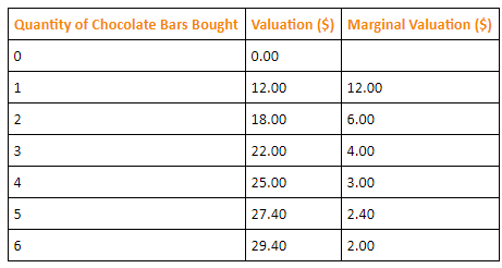
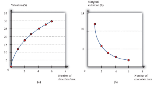
Note: Your valuation of a good is the maximum amount that you would be willing to pay, purely on the basis of your desire for the good.
Because you are willing to pay $12 for one bar and $18 for two bars, we know you would be willing to pay an additional $6 for the second chocolate bar. Similarly, if you have two chocolate bars, you would be willing to pay an additional $4 for a third bar. We call the change in your valuation your marginal valuation (see the third column of the Table above "Valuation and Marginal Valuation", which is graphed in part [b] of the Figure above "Valuation of a Good"). Notice that marginal valuation decreases as the quantity of chocolate bars increases. The change in your valuation gets smaller as you obtain more chocolate bars. We can see the same thing in part (a) of the Figure above "Valuation of a Good" from the fact that the valuation curve gets flatter as the quantity of chocolate bars increases.
It usually seems reasonable to think that marginal valuations will indeed decrease in this way. If you don’t have any chocolate bars, then the first bar is worth a lot to you—$12 in our example. But if you already have five chocolate bars, then the sixth bar is worth only $2 to you. As you obtain more and more of any given product, each additional unit is less and less valuable. For most people, we expect that most products will exhibit such diminishing marginal valuation.
Part (b) of the Figure "Valuation of a Good" may seem familiar. It is the demand curve for chocolate bars you saw previously in the Figure "The Demand Curve". This is not an accident or a coincidence. There is a simple decision rule to tell you how much you should buy: when your marginal valuation is greater than the price, you should buy more of the good, stopping only when the marginal valuation of the good has dropped to the level of the price. For example, suppose that chocolate bars are selling for $3.99. You should definitely buy the first chocolate bar, because it is worth $10 to you and will cost you only $3.99. You should buy the second bar as well because it is worth an additional $8 to you; likewise you should buy the third and fourth bars. You don’t buy the fifth bar because it is worth only $3 to you, which is less than what it costs. Thus your decision rule is as follows:
- Buy until the marginal valuation of a good equals the price of the good.
Because the demand curve, by definition, tells you how much you buy at a given price, it is the same as the marginal valuation curve.
- Buy until the marginal valuation of a good equals the price of the good.
7. Making Decisions at the Margin
- To make good decisions, you need to understand the trade-offs you are making. To put it another way, you need to recognize that every purchase has an opportunity cost, which is summarized by the budget line. If you want more chocolate bars, you must consume less of something else. You also need to find the right point on the budget line—the point that makes you happiest. Most of the time, economists simply assume that you are able to make this decision correctly on the basis of the three assumptions about your preferences that we introduced earlier.
- You can also use this theory to help you think about the decisions you make. Suppose you are facing the budget line we discussed earlier and plan to buy 8 chocolate bars and 60 downloads (as in the Figure "Choosing a Preferred Point on the Budget Line"). In principle, you need to compare that bundle with every other combination on the budget line. In practice, it is enough—most of the time at least—to compare it with nearby bundles. For example, if you prefer this bundle to 7 chocolate bars and 65 downloads, and you also prefer this bundle to 9 chocolate bars and 55 downloads, then you can be reasonably confident that you have found the best bundle. If a small change won’t make you happier, then neither will a large change.
8. Unit Demand
- So far we have considered situations where you might buy multiple units of a good—for example, 20 music downloads or 5 chocolate bars. To keep things simple, we also supposed that you could buy fractional amounts, such as 20.7 downloads, or 3.25 chocolate bars. This assumption gives a decision rule for purchase: buy until marginal valuation equals price.
- Some purchase decisions are better thought of as “buy or don’t buy.” Large, infrequent purchases fall into this category. Think, for example, about the decision to buy a new car, a new microwave, or an expensive vacation. You won’t buy five microwaves because they are cheap. The decision rule for purchase is even easier in this case: buy if your valuation of the good exceeds the price of the good. In fact, this is really no different from our earlier decision rule. Because you are only ever thinking about buying one unit, your valuation and your marginal valuation are the same thing (look back at the first two rows of the Table "Valuation and Marginal Valuation"). And because in this case it does not make sense to suppose you can buy fractional amounts of the good, you cannot keep buying until your marginal valuation decreases all the way to the price.
- If a buyer is interested in purchasing one and only one unit of a good, the unit demand curve tells us the price at which he is willing to buy. Below his valuation, he buys the good. Above his valuation, he does not buy the good. A unit demand curve is shown in the Figure below "Unit Demand". In this example, the buyer’s valuation is $3,000.
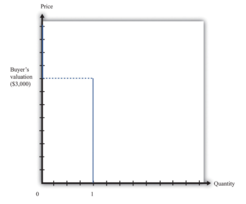
Note: The buyer follows this decision rule: “Buy if the price is less than valuation.” If the price is greater than $3,000, the buyer will not purchase. The quantity demanded is zero. If the price is less than $3,000, the buyer will purchase one unit. No matter how low the price decreases, the buyer will not want more than a single unit. This is an example of unit demand.
To see where such a valuation could come from, look at the Figure below "The Valuation of a Car". Suppose you are thinking about buying a car. The figure shows our standard downloads-and-chocolate-bar diagram, except that there are two budget lines. The outer budget line applies in the case where you do not buy the car. You have a preferred point in terms of downloads and chocolate bars (A). If you buy the car, you have less income to spend on everything else. The effect is to shift your budget line inward, in which case you have a new preferred point (B). The thought experiment here is to decrease your income and shift your budget line inward until you are equally happy with the two bundles. The change in your income—the amount by which the budget line must shift—is your valuation of the car. Your valuation, in other words, is the opportunity cost of the car: if you buy the car, you can only consume bundle B rather than bundle A.
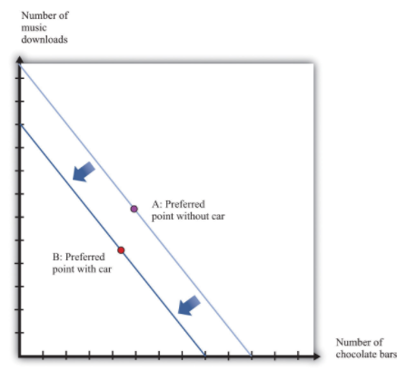
Note: If you don’t buy a car, your preferred mix of chocolate bars and downloads is at point A. If you buy a car, then you no longer have that income available to spend on chocolate bars and downloads. Your budget line shifts inward, and you consume at your preferred point B. Now imagine that you are equally happy at point A and point B. Then the difference in income is equal to your valuation of the car. Thus the valuation of a car is its opportunity cost in terms of other goods.
9. Budget Studies
- Economists’ theories are all well and good. But we do not actually get to see people’s preferences or marginal valuations. We observe what people actually do. To see our theory in action, we can look at household budget studies. These are surveys where government statisticians interview households and ask them how they spend their income. For example, the Table below "Budget Shares in the United States" contains data on US consumer expenditures for the years 2005, 2007, and 2009.
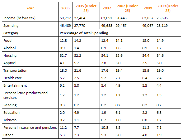
You can see that, on average, households spend a little more than 45 percent of their income on food and housing. Insurance is also a large category, with about 11 percent of income being spent on it. From this we see that, although individual goods may be inferior or luxury goods, such differences are largely offset when we look at broad categories of goods or services. The table also contains data for households under age 25.This is based on the age of the reference person in the household, who is the individual who owns or rents the property. We can compare the spending patterns of this group against all households. Not surprisingly, the younger group earns less than the average household. Also, this younger group often spends more than it earns, indicating that younger people are borrowing, on average. The younger group spends more on alcohol, transportation, and education and much less on health care and insurance than the average household. This makes sense given the health status of young individuals as well as their demand for education.
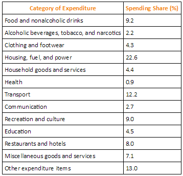
The Table below "United Kingdom Budget Study" is a UK budget study for households headed by young people (under the age of 30) in 2009. It shows how these households allocated their expenditures over a week.The British source is as follows: Office for National Statistics, Family Spending, 2010,table A.11, accessed January 24, 2011, http://www.statistics.gov.uk/downloads/theme_social/family-spending-2009/familyspending2010.pdf. We can compare these figures against those for young people in the United States. (We need to be careful in making comparisons because the categories for spending are not exactly the same across surveys. Still, it is useful to explore these differences.) In the United Kingdom, spending on food and housing is much lower for these younger households than in the United States. Health also has a much lower expenditure share.
Last modified: Tuesday, August 14, 2018, 10:08 AM