Reading: An Introduction to Relational Database Theory
1 Introduction
1.1 Introduction
This chapter gives a very broad overview of
• what a database is
• what a relational database is, in particular
• what a database management system (DBMS) is
• what a DBMS does
• how a relational DBMS does what a DBMS does
We start to familiarise ourselves with terminology and notation used in the remainder of the book, and we get a brief introduction to each topic that is covered in more detail in later sections.
1.2 What Is a Database?
You will find many definitions of this term if you look around the literature and the Web. At one time (in 2008), Wikipedia [1] offered this: “A structured collection of records or data.” I prefer to elaborate a little:
A database is an organized, machine-readable collection of symbols, to be interpreted as a true account of some enterprise. A database is machine-updatable too, and so must also be a collection of variables. A database is typically available to a community of users, with possibly varying requirements.
The organized, machine-readable collection of symbols
is what you “see” if you “look at” a database at a particular point in time. It is to be
interpreted as a true account of the enterprise at that point in time. Of course it might happen to be incorrect,
incomplete or inaccurate, so perhaps it is better to say that the account is believed to be true.
The alternative view of a database as a collection of variables reflects the fact that the account of the enterprise has to change from time to time, depending on the frequency of change in the details we choose to include in that account.
The suitability of a particular kind of database (such as relational, or object-oriented) might depend to some extent on the requirements of its user(s). When E.F. Codd developed his theory of relational databases (first published in 1969), he sought an approach that would satisfy the widest possible ranges of users and uses. Thus, when designing a relational database we do so without trying to anticipate specific uses to which it might be put, without building in biases that would favour particular applications. That is perhaps the distinguishing feature of the relational approach, and you should bear it in mind as we explore some of its ramifications.
1.1 “Organized Collection of Symbols”
For example, the table in Figure 1.1 shows an organized collection of symbols.
|
StudentId |
Name |
CourseId |
|
S1 |
Anne |
C1 |
|
S1 |
Anne |
C2 |
|
S2 |
Boris |
C1 |
|
S3 |
Cindy |
C3 |
Figure 1.1: An Organized Collection of Symbols
Can you guess what this tabular arrangement of symbols might be trying to tell us? What might it mean, for symbols to appear in the same row? In the same column? In what way might the meaning of the symbols in the very first row (shown in blue) differ from the meaning of those below them?
Do you intuitively guess that the symbols below the first row in the first column are all student identifiers, those in the second column names of students, and those in the third course identifiers? Do you guess that student S1’s name is Anne? And that Anne is enrolled on courses C1 and C2? And that Cindy is enrolled on neither of those two courses? If so, what features of the organization of the symbols led you to those guesses?
Remember those features. In an informal way they form the foundation of relational theory. Each of them has a formal counterpart in relational theory, and those formal counterparts are the only constituents of the organized structure that is a relational database.
1.2 “To Be Interpreted as a True Account”
For example (from Figure 1.1):
|
StudentId |
Name |
CourseId |
|
S1 |
Anne |
C1 |
Perhaps those green symbols, organized as they are with respect to the blue ones, are to be understood to mean:
“Student S1, named Anne, is enrolled on course C1.”
An important thing to note here is that only certain symbols from the sentence in quotes appear in the table—S1, Anne, and C1. None of the other words appear in the table. The symbols in the top row of the table (presumably column headings, though we haven’t actually been told that) might help us to guess “student”, “named”, and “course”, but nothing in the table hints at “enrolled”. And even if those assumed column headings had been A, B and C, or X, Y and Z, the given interpretation might still be the intended one.
Now, we can take the sentence “Student S1, named Anne, is enrolled on course C1” and replace each of S1, Anne, and C1 by the corresponding symbols taken from some other row in the table, such as S2, Boris, and C1. In so doing, we are applying exactly the same mode of interpretation to each row. If that is indeed how the table is meant to be interpreted, then we can conclude that the following sentences are all true:
Student S1, named Anne, is enrolled on course C1. Student S1, named Anne, is enrolled on course C2. Student S2, named Boris, is enrolled on course C1. Student S3, named Cindy, is enrolled on course C3.
In Chapter 3, “Predicates and Propositions”, we shall see exactly how such interpretations can be systematically formalized. In Chapter 4, “Relational Algebra—The Foundation”, and Chapter 5, “Building on The Foundation”, we shall see how they help us to formulate correct queries to derive useful information from a relational database.
1.1 “Collection of Variables”
Now look at Figure 1.2, a slight revision of Figure 1.1.
ENROLMENT
|
StudentId |
Name |
CourseId |
|
S1 |
Anne |
C1 |
|
S1 |
Anne |
C2 |
|
S2 |
Boris |
C1 |
|
S3 |
Cindy |
C3 |
|
S4 |
Devinder |
C1 |
Figure 1.2: A variable, showing its current value
We have added the name, ENROLMENT, above the table, and we have added an extra row.
ENROLMENT is a variable. Perhaps the table we saw earlier was once its value. If so, it (the variable) has been updated since then—the row for S4 has been added. Our interpretation of Figure 1.1 now has to be revised to include the sentence represented by that additional row:
Student S1, named Anne, is enrolled on course C1. Student S1, named Anne, is enrolled on course C2. Student S2, named Boris, is enrolled on course C1. Student S3, named Cindy, is enrolled on course C3. Student S4, named Devinder, is enrolled on course C1.
Notice that in English we can join all these sentences together to form a single sentence, using conjunctions like “and”, “or”, “because” and so on. If we join them using “and” in particular, we get a single sentence that is logically equivalent to the given set of sentences in the sense that it is true if each one of them is true (and false if any one of them is false). A database, then, can be thought of as a representation of an account of the enterprise expressed as a single sentence! (But it’s more usual to think in terms of a collection of individual sentences.)
We might also be able to conclude that the following sentences (for example) are false:
Student S2, named Boris, is enrolled on course C2. Student S2, named Beth, is enrolled on course C1.
Whenever the variable is updated, the set of true sentences represented by its value changes in some way. Updates usually reflect perceived changes in the enterprise, affecting our beliefs about it and therefore our account of it.
1.1 What Is a Relational Database?
A relational database is one whose symbols are organized into a collection of relations. Figure 1.3 confirms that the examples we have already seen are in fact relations, depicted in tabular form. Indeed, according to Figure 1.2, the relation depicted in Figure 1.3 is the current value of the variable ENROLMENT.
|
StudentId |
Name |
CourseId |
|
S1 |
Anne |
C1 |
|
S1 |
Anne |
C2 |
|
S2 |
Boris |
C1 |
|
S3 |
Cindy |
C3 |
|
S4 |
Devinder |
C1 |
Figure 1.3: A relation, shown in tabular form
Happily, the visual (tabular) representation we have been using thus far is suited particularly well to relational databases: so much so that many people use the word table as an alternative to relation. The language SQL in particular uses that term, so in the context of relational theory it is convenient and judicious to stick with relation for the theoretical construct, allowing SQL’s deviations from relational theory to be noted as differences between tables and relations.
Relation is a formal term in mathematics—in particular, in the logical foundation of mathematics. It appeals to the notion of relationships between things. Most mathematical texts focus on relations involving things taken in pairs but our example shows a relation involving things taken three at a time and, as we shall see, relations in general can relate any number of things (and, as we shall see, the number in question can even be less than two, making the term relation seem somewhat inappropriate).
Relational database theory is built around the concept of a relation. Our study of the theory will include:
• The “anatomy” of a relation.
• Relational algebra: a set of mathematical operators that operate on relations and yield relations as results.
• Relation variables: their creation and destruction, and operators for updating them.
• Relational comparison operators, allowing consistency rules to be expressed as constraints
(commonly called integrity constraints) on the variables constituting the database.
And we will see how these, and other constructs, can form the basis of a database language (specifically, a relational database language).
1.2 “Relation” Not Equal to “Table”
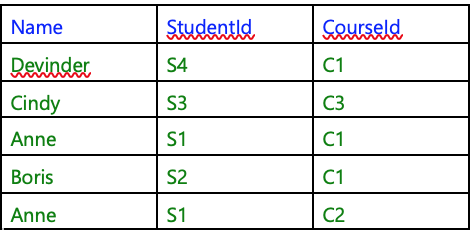
“Table”, here, refers to pictures of the kind shown in Figures 1.1, 1.2, and 1.3. The terms relation and table are not synonymous. For one thing, although every relation can be depicted as a table, not every table is a representation of (i.e., denotes) some relation. For another, several different tables can all represent the same relation. Consider Figure 1.4, for example.
(Actually, there are two very special relations which cannot sensibly be depicted in tabular form.)
Figure 1.4: Same relation as Figure 1.3
The table in Figure 1.4 is different from the one in Figure 1.3, but it represents the same relation. I have changed the order of the columns and the order of the rows, each green row in Figure 1.4 has the same symbols for each column heading as some row in Figure 1.3 and each row in Figure 1.3 has a corresponding row, derived in that way, in Figure 1.4. What I am trying to illustrate is the principle that the relation represented by a table does not depend on the order in which we place the rows or the columns in that table. It follows that several different tables can all denote the same relation, because we can simply change the left-to-right order in which the columns are shown and/or the top-to-bottom order in which the rows are shown and yet still be depicting the same relation.
What does it mean to say that the order of columns and the order of rows doesn’t matter? We will find out the answer to this question when we later study the typical operators that are defined for operating on relations (e.g., to compute results of queries against the database) and relation variables (e.g., to update the database). None of these operators will depend on the notion of some row or some column being the first or last, or immediately before or after some other column or row.
We can also observe that not every table depicts a relation. Such tables can easily be obtained just by deleting the blue rows (the column headings) from each of Figures 1.1 to 1.4. Figure 1.5 shows another table that does not depict any relation.
|
A |
B |
A |
|
1 |
2 |
3 |
|
4 |
|
5 |
|
6 |
7 |
8 |
|
9 |
9 |
? |
|
1 |
2 |
3 |
Figure 1.5: Not a relation
The various reasons why this table cannot be depicting a relation should become apparent to you by the time you reach the end of this chapter.
1.1 Anatomy of a Relation
Figure 1.6 shows the terminology we use to refer to parts of the structure of a relation.
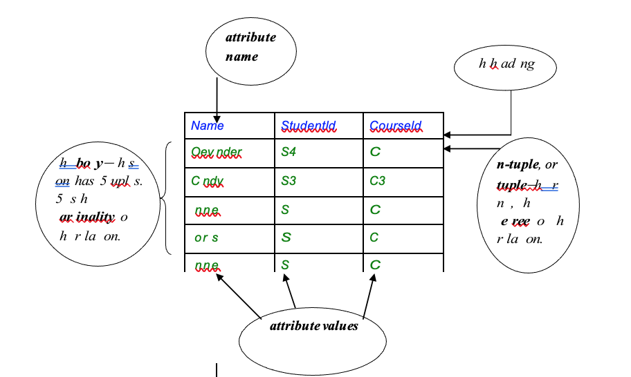
Figure 1.6: Anatomy of a relation
Because of the distinction I have noted between the terms relation and table, we prefer not to use the terminology of tables for the anatomical parts of a relation. We use instead the terms proposed by
E.F. Codd, the researcher who first proposed relational theory as a basis for database technology, in 1969.
Try to get used to these terms. You might not find them very intuitive. Their counterparts in the tabular representation might help:
• relation : table
• (n-)tuple : row
• attribute : column Also (as shown in Figure 1.6):
The degree is the number of attributes. The cardinality is the number of tuples.
The heading is the set of attributes (note set, because the attributes are not ordered in any way and no attribute appears more than once).
The body is the set of tuples (again, note set—the tuples are not ordered and no tuple appears more than once).
An attribute has an attribute name, and no two have the same name. Each attribute has an attribute value in each tuple.
1.1 What Is a DBMS?
A database management system (DBMS) is exactly what its name suggests—a piece of software for managing databases and providing access to them. But be warned!—in the industry the term database is commonly used to refer to a DBMS, especially in promotional literature. You are strongly discouraged from adopting such sloppy practice (if such a system is a database, what are the things it manages?)
A DBMS responds to commands given by application programs, custom-written or general-purpose, executing on behalf of users. Commands are written in the database language of the DBMS (e.g., SQL). Responses include completion codes, messages and results of queries.
In order to support multiple concurrent users a DBMS normally operates as a server. Its immediate users are thus those application programs, running as clients of this server, typically (though not necessarily) on behalf of end users. Thus, some kind of communication protocol is needed for the transmission of commands and responses between client and server. Before submitting commands to the server a client application program must first establish a connection to it, thus initiating a session, which typically lasts until the client explicitly asks for it to be terminated. That is all you need to know about client-server architecture as far as this book is concerned.
This book is concerned with relational DBMSs and relational databases in particular, and soon we will be looking at the components we expect to find in a relational DBMS. Before that we need to briefly review what is expected of a DBMS in general.
1.1 What Is a Database Language?
To repeat, the commands given to a DBMS by an application are written in the database language of the DBMS. The term data sublanguage is sometimes used instead of database language. The sub- prefix refers to the fact that application programs are sometimes written in some more general-purpose programming language (the “host” language), in which the database language commands are embedded in some prescribed style. Sometimes the embedding style is such that the embedded statements are unrecognized by the host language compiler or interpreter, and some special preprocessor is used to replace the embedded statements by, for example, CALL statements in the host language.
A query is an expression that, when evaluated, yields some result derived from the database. Queries are what make databases useful. Note that a query is not of itself a command (though some texts, curiously, use the term query for commands as well as genuine queries, including commands that update the database!). The DBMS might support some kind of command to evaluate a given query and make the result available for access, also using DBMS commands, by the application program. The application program might execute such commands in order to display a query result (usually in tabular form) in a window.
1.2 What Does a DBMS Do?
In response to requests from application programs, we expect a DBMS to be able, for example, to
• create and destroy variables in the database
• take note of integrity rules (constraints)
• take note of authorisations (who is allowed to do what, to what)
• update variables (honouring constraints and authorisations)
• provide results of queries
To amplify some of the terms just used:
The requests take the form of commands written in the database language supported by the DBMS.
The variables are the constituents of the database, like the ENROLMENT variable we looked at earlier. Such variables are both persistent and global. A persistent variable is one that ceases to exist only when its destruction is explicitly requested by some user. A global variable is one that exists independently of the application programs that use it, distinguishing it from a local variable, declared within the application program and automatically destroyed when the program unit (“block”) in which it is declared finishes its execution.
Constraints (sometimes called integrity constraints) are rules governing permissible values, and permissible combinations of values, of the variables. For example, it might be possible to tell the DBMS that no student’s assessment score can be less than zero. A database that violates a constraint is, by definition, incorrect—it represents an account that is in some respect false. A database that satisfies all its constraints is said to be consistent, even though it cannot in general be guaranteed to be correct.
In the sense that constraints are for integrity, authorisations are for security. Some of the data in a database might represent sensitive information whose accessibility is restricted to certain privileged users only. Similarly, it might be desired to allow some users to access certain parts of the database without also being able to update those parts.
Note the three parts of an authorisation: who, what, and to what. “Who” is a user of the database; “what” is one of the operations that are available for operating on the variables in the database; “to what” is one of those variables.
In the remaining sections of this chapter you will see examples of how a relational DBMS does these things. Unless otherwise stated, the examples use commands written in Tutorial D.
1.1 Creating and Destroying Variables
Example 1.1 shows a command to create the variable shown in Figure 1.2:
Example 1.1: Creating a database variable.
VAR ENROLMENT BASE RELATION
{ StudentId SID , Name CHAR , CourseId CID }
KEY { StudentId, CourseId } ;
Explanation 1.1:
VAR is a key word, indicating that a variable is to be created.
ENROLMENT is the variable’s name.
BASE is a key word indicating that the variable is to be part of the database, thus both persistent and global. If BASE were omitted, then the command would result in creation of a local variable.
The text from RELATION to the closing brace specifies the declared type of the variable, meaning that every value ever assigned to ENROLMENT must be a value of that type.
The declared type of ENROLMENT is a relation type, indicated by the key word RELATION and a heading specification. Thus, every value ever assigned to ENROLMENT must be a relation of that type. A heading specification consists of a list of attribute names, each followed by a type name, the entire list being enclosed in braces. Thus, each attribute of the heading also has a declared type. The type names SID and CID (for student ids and course ids) refer to user- defined types. User-defined types have to be defined by some user of the DBMS before they can be referred to. The type name CHAR (character strings), by contrast, is a built-in type: it is provided by the DBMS itself, is available to all users, and cannot be destroyed.
Chapter 2, “Values, Types, Variables, Operators”, deals with types in more detail, and shows you how to define types such as SID and CID.
KEY indicates that the variable is subject to a certain kind of constraint, in this case declaring that no two tuples in the relation assigned to ENROLMENT can ever have the same combination of attribute values for StudentId and CourseId (i.e., we cannot enrol the same student on the same course more than once, so to speak). We will learn more about constraints in general and key constraints in particular in Chapter 6.
Destruction of ENROLMENT is the simple matter shown in Example 1.2,
Example 1.2: Destroying a variable.
DROP VAR ENROLMENT ;
After execution of this command the variable no longer exists and any attempt to reference it is in error.
1.1 Taking Note of Integrity Rules
For example, suppose the university has a rule to the effect that there can never be more than 20,000 enrolments altogether. Example 1.3 shows how to declare the corresponding constraint in Tutorial D.
Example 1.3: Declaring an integrity constraint.
CONSTRAINT MAX_ENROLMENTS
COUNT ( ENROLMENT ) 20000 ;
Explanation 1.3:
• CONSTRAINT is the key word indicating that a constraint is being declared.
• MAX_ENROLMENTS is the name of the constraint.
• COUNT ( ENROLMENT ) is a Tutorial D expression yielding the cardinality (see the earlier section, “Anatomy of a Relation”) of the current value of ENROLMENT.
• COUNT (ENROLMENT) --> 20000 is a truth-valued expression, yielding true if the cardinality is less than or equal to 20000, otherwise yielding false. (Note regarding Rel: Because the symbol --> is normally unavailable on keyboards, Rel accepts <= in its place.)
The declaration tells the DBMS that the database is inconsistent if the value of MAX_ENROLMENTS is ever false, and that the DBMS is therefore to reject any attempt to update the database that, if accepted, would bring about that situation.
Example 1.4 shows how to retract a constraint that ceases to be applicable.
Example 1.4: Retracting an integrity constraint.
DROP CONSTRAINT MAX_ENROLMENTS ;
1.1 Taking Note of Authorisations
Tutorial D does not include any commands for creating and destroying permissions, because security and authorization, though important, are not specifically relational database issues. If Tutorial D did include such commands, we might reasonably expect them to look like those shown in Example 1.5, which are meant to be self-explanatory.
Example 1.5: Creating permissions
PERMISSION U9_ENROLMENT FOR User9 TO READ ENROLMENT ; PERMISSION U8_ENROLMENT FOR User8 TO UPDATE ENROLMENT ;
Note the syntactic consistency with commands we have already seen: a key word indicating the kind of thing being created or destroyed, followed by the name of the thing, followed in turn by the specification of the thing. (C.J. Date, co-designer of Tutorial D, makes a slightly different suggestion for granting permissions in his Introduction to Database Systems, 8th edition, on page 506.)
How do you rate computer languages you are already acquainted with, for syntactic consistency? For example, the database language SQL has been noted to suffer from several syntactic inconsistencies (as well as—much more seriously—several harmful deviations from relational database theory).
By now you can predict the command, consistent with Example 1.5 and shown in Example 1.6, to be used to retract a permission previously granted.
Example 1.6: Retracting a permission
DROP PERMISSION U9_ENROLMENT ;
In case you are familiar with SQL’s GRANT and REVOKE statements that are used for such purposes, you might like to give some thought to the advantages and disadvantages of using specific names for permissions. SQL doesn’t use them—in an SQL REVOKE statement you have to repeat the details of the permission you are withdrawing.
1.1 Updating Variables
The usual way of updating a variable in computer languages is by assignment. For example, if X is an integer variable, the assignment X := X + 1 updates X such that its value immediately after execution of the assignment is one more than its value was immediately beforehand. The expression on the right of := denotes the source for the assignment and the variable name on the left denotes the target.
When the target is a relation variable—as it always is when it is part of a relational database—the source must be a relation. You will learn how to write expressions that denote relations in Chapters 2, 4 and 5, but in any case assignment, though it should be available (it isn’t in SQL), is not the usual way of applying updates to a relational database. This is because there is very often only a small amount of difference, in a manner of speaking, between the “old” value and the “new” value and it is usually much more convenient to be able to express the update in terms of that small difference.
The differential update operators expected in a relational DBMS are usually called INSERT, DELETE, and UPDATE, and those are the names used in Tutorial D (also in SQL). Take a look at DELETE first (Example 1.8).
Example 1.8: Updating by deletion
DELETE ENROLMENT WHERE StudentId = SID ( 'S4' ) ;
Explanation 1.8:
• Informally, Example 1.8 deletes all the tuples for student S4 and can be interpreted as meaning “student S4 is no longer enrolled on any courses”. More formally, it assigns to the variable ENROLMENT the relation whose body consists of those tuples in the current value of ENROLMENT that fail to satisfy the condition given in the WHERE clause—thus, every tuple in which the value of the StudentId attribute is not the student identifier S4.
• StudentId = SID ( 'S4' ) is a conditional expression. Because it follows the key word WHERE here, it is in fact a WHERE condition, also known as a restriction condition.
• The expression SID ( 'S4' ) will be explained in Chapter 2, when we study types.
Next, in Example 1.9, we look at UPDATE.
Example 1.9: Updating by replacement
UPDATE ENROLMENT WHERE StudentId = SID ( 'S1' ) :
{ Name := 'Ann' } ;
Note that UPDATE uses a WHERE clause, just like DELETE. The WHERE clause is followed by a list of assignments—in Example 1.9 just one assignment—but these are assignments to attributes, not assignments to variables.
Explanation 1.9:
• Informally, Example 1.9 updates each ENROLMENT tuple for student S1, changing its Name value to 'Ann'. More formally, it assigns to the variable ENROLMENT the relation that is identical to the current value in all respects except that the value for the attribute Name, in the tuples whose StudentId value is the student identifier S1, becomes the string 'Ann' in each case. (I would have written “except possibly” had I not known that the existing Name value in those tuples is 'Anne' in each case. In some circumstances no change takes place as a result of executing an UPDATE, and the same applies to DELETE and INSERT.)
• Name := 'Ann' is an attribute assignment. An attribute assignment sets the value of the target attribute to the specified value, in each tuple that satisfies the WHERE condition.
Finally, Example 1.10 illustrates the use of INSERT.
Example 1.10: Updating by insertion
INSERT ENROLMENT RELATION {
TUPLE { StudentId SID ( 'S4' ) ,
Name 'Devinder' ,
CourseId CID ( 'C1' ) } } ;
Explanation 1.10:
• Informally, Example 1.10 adds a tuple to ENROLMENT indicating that student S4, still called Devinder, is now enrolled on course C1. More formally, it assigns to the variable ENROLMENT the relation consisting of every tuple in the current value of ENROLMENT and every tuple (there is only one in this particular example) in the relation denoted by the expression following the word ENROLMENT.
• The expression beginning with the key word TUPLE and ending at the penultimate closing brace denotes the tuple consisting of the three indicated attribute values:
SID ( 'S4' ) for the attribute StudentId, 'Devinder' for the attribute Name, and CID ( 'C1' ) for the attribute CourseId.
• The expression beginning with the key word RELATION and ending at the final closing brace denotes the relation whose body consists of that single tuple. Such expressions are fully explained in Chapter 2, “Values, Types, Variables, Operators”.
Example 1.8 has no effect on the database in the case where the current value of ENROLMENT has no tuples for student S4.
Example 1.9 has no effect on the database in the case where the current value of ENROLMENT has no tuples for student S1.
Example 1.10 has no effect on the database in the case where the current value of ENROLMENT already contains the tuple representing the enrolment of student S4, named Devinder, on course C1. It also has no effect on the database if the cardinality of the current value of ENROLMENT is 20,000 and the constraint MAX_ENROLMENTS (Example 1.3) is in effect. In this case, and possibly in the first case too, an error message results.
1.1 Providing Results of Queries
Expressing queries in Tutorial D is the (big) subject of Chapters 4 and 5. Here I present just a simple example to give you the flavour of things to come in those chapters. Example 1.11 is a query expressing the question, who is enrolled on course C1?
Example 1.11: A query in Tutorial D
ENROLMENT WHERE CourseId = CID('C1')
{ StudentId, Name }
Note carefully that Example 1.11 is not a command. It is just an expression, denoting a value—in this case, a relation. In a relational database language the result of a query is always another relation! Figure 1.7 shows the result of Example 1.11 in the usual tabular form.
|
StudentId |
Name |
|
S1 |
Anne |
|
S2 |
Boris |
|
S4 |
Devinder |
Explanation 1.11:
Figure 1.7: Result of query in Example 1.11
• WHERE is the key word identifying the Tutorial D operator of that name. This operator operates on a given relation and yields a relation. Certain operators, including this one, that operate on relations and yield relations together constitute the relational algebra, covered in detail in Chapter 4.
• CourseId = CID('C1') qualifies WHERE, specifying that just the tuples for course C1 are required.
• { StudentId, Name } specifies that from the result of the previous operation (WHERE) just the StudentId and Name attributes are required.
The overall result is a relation formed from the current value of ENROLMENT by discarding certain tuples and a certain attribute.
EXERCISE
Consider the table shown in Figure 1.5, repeated here for convenience:
|
A |
B |
A |
|
1 |
2 |
3 |
|
4 |
|
5 |
|
6 |
7 |
8 |
|
9 |
9 |
? |
|
1 |
2 |
3 |
Give three reasons why it cannot possibly represent a relation. By the way, this table is supported by SQL, and the three reasons represent some of SQL’s serious and far-reaching deviations from relational theory.
Остання зміна: понеділок 13 червня 2022 09:43 AM