Reading: Lesson 1 - Time Value Money & Future Values
4.1.A - Time Value Money & Future Values
1. Time Value Money
- The primary objective of financial management is to maximize the intrinsic value of a firm’s stock. We also saw that stock values depend on the timing of the cash flows investors expect from an investment—a dollar expected sooner is worth more than a dollar expected further in the future. Therefore, it is essential for financial managers to understand the time value of money and its impact on stock prices.
- The principles of time value analysis have many applications, including retirement planning, loan payment schedules, and decisions to invest (or not) in new equipment. In fact, of all the concepts used in finance, none is more important than the time value of money (TVM), also called discounted cash flow (DCF) analysis.
- The first step in a time value analysis is to set up a time line to help you visualize what’s happening in the particular problem. To illustrate, consider the following diagram, where PV represents $100 that is in a bank account today and FV is the value that will be in the account at some future time (3 years from now in this example):
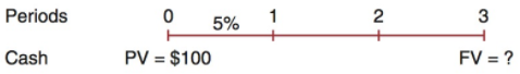
4. The intervals from 0 to 1, 1 to 2, and 2 to 3 are time periods such as years or months. Time 0 is today, and it is the beginning of Period 1; Time 1 is one period from today, and it is both the end of Period 1 and the beginning of Period 2; and so on. In our example, the periods are years, but they could also be quarters or months or even days. Note again that each tick mark corresponds to both the end of one period and the beginning of the next one. Thus, if the periods are years, the tick mark at Time 2 represents both the end of Year 2 and the beginning of Year 3.
5. Cash flows are shown directly below the tick marks, and the relevant interest rate is shown just above the time line. Unknown cash flows, which you are trying to find, are indicated by question marks. Here the interest rate is 5%; a single cash outflow, $100, is invested at Time 0; and the Time-3 value is unknown and must be found. In this example, cash flows occur only at Times 0 and 3, with no flows at Times 1 or 2. We will, of course, deal with situations where multiple cash flows occur. Note also that in our example the interest rate is constant for all 3 years. The interest rate is generally held constant, but if it varies, then in the diagram we show different rates for the different periods.
2. Future Values
- A dollar in hand today is worth more than a dollar to be received in the future—if you had the dollar now you could invest it, earn interest, and end up with more than one dollar in the future. The process of going forward, from present values (PVs) to future values (FVs), is called compounding. To illustrate, refer back to our 3-year time line and assume that you have $100 in a bank account that pays a guaranteed 5% interest each year. How much would you have at the end of Year 3? We first define some terms, and then we set up a time line and show how the future value is calculated.
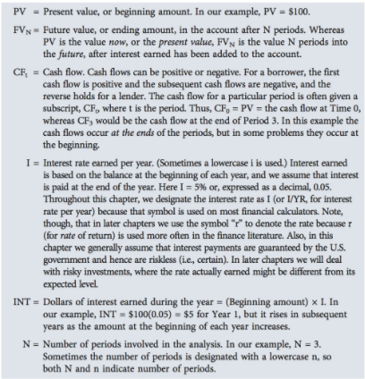
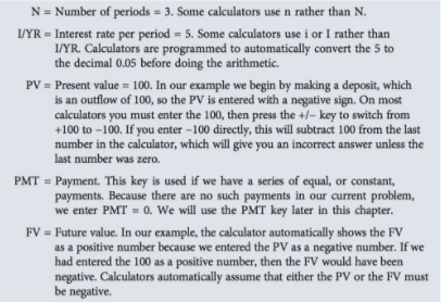
2. The time line itself can be modified and used to find the FV of $100 compounded for 3 years at 5%, as shown below:
![]()
3. We start with $100 in the account, which is shown at t = 0. We then multiply the initial amount, and each succeeding beginning-of-year amount, by (1 + I) = (1.05). • You earn $100(0.05) = $5 of interest during the first year, so the amount at the end of Year 1 (or at t = 1) is
4. We begin the second year with $105, earn 0.05($105) = $5.25 on the now larger beginning-of-period amount, and end the year with $110.25. Interest during Year 2 is $5.25, and it is higher than the first year’s interest, $5, because we earned $5(0.05) = $0.25 interest on the first year’s interest. This is called “compounding,” and interest earned on interest is called “compound interest.
5. This process continues, and because the beginning balance is higher in each successive year, the interest earned each year increases. The total interest earned, $15.76, is reflected in the final balance, $115.76.
6. The step-by-step approach is useful because it shows exactly what is happening. However, this approach is time-consuming, especially if the number of years is large and you are using a calculator rather than Excel, so streamlined procedures have been developed.
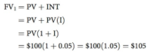
7. In the step-by-step approach, we multiplied the amount at the beginning of each period by (1 + I) = (1.05). Notice that the value at the end of Year 2 is
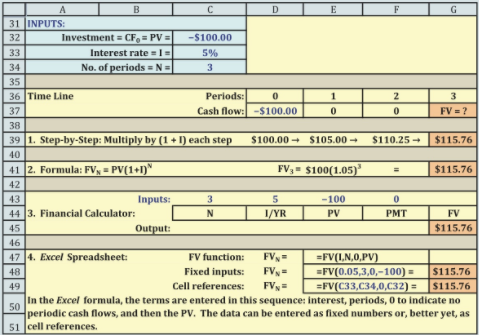
8. N = 3, then we multiply PV by (1 + I) three different times, which is the same as multiplying the beginning amount by (1 + I)3. This concept can be extended, and the result is this key equation
![]()
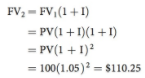
9. We can apply this equation to find the FV in our example:
![]()
3. Financial Calculators and Spreadsheets
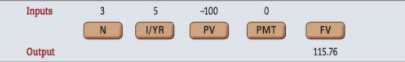
- Financial calculators were designed specifically to solve time value problems. First, note that financial calculators have five keys that correspond to the five variables in the basic time value equations. The previous equation has only four variables, but we will shortly deal with situations where a fifth variable (a set of periodic additional payments) is involved. We show the inputs for our example above their keys in the following diagram, and the output, which is the FV, below its key. Because there are no periodic payments in this example, we enter 0 for PMT.
2. Spreadsheets are ideally suited for solving many financial problems, including those dealing with the time value of money.2 Spreadsheets are obviously useful for calculations, but they can also be used like a word processor to create exhibits like the figure above, which includes text, drawings, and calculations. We use this figure to show that four methods can be used to find the FV of $100 after 3 years at an interest rate of 5%. The time line on Rows 36 to 37 is useful for visualizing the problem, after which the spreadsheet calculates the required answer. Note that the letters across the top designate columns, the numbers down the left column designate rows, and the rows and columns jointly designate cells. Thus, cell C32 shows the amount of the investment, $100, and it is given a minus sign because it is an outflow.
3. On Row 39, we go through the step-by-step calculations, multiplying the beginning-of-year values by (1 + I) to find the compounded value at the end of each period. Cell G39 shows the final result of the step-by-step approach. We illustrate the formula approach in Row 41 to find the FV. Cell G41 shows the formula result, $115.76. As it must, it equals the step-by-step result. Rows 43 to 45 illustrate the financial calculator approach, which again produces the same answer, $115.76. The last section, in Rows 47 to 49, illustrates Excel’s future value (FV) function. You can access the function wizard by clicking the fx symbol in Excel’s formula bar. Then select the category for Financial functions, and then the FV function, which is =FV(I,N,0,PV), as shown in Cell E47.3 Cell E48 shows how the formula would look with numbers as inputs; the actual function itself is entered in Cell G48, but it shows up in the table as the answer, $115.76. If you access the model and put the pointer on Cell G48, you will see the full formula. Finally, Cell E49 shows how the formula would look with cell references rather than fixed values as inputs, with the actual function again in Cell G49. We generally use cell references as function inputs because this makes it easy to change inputs and see how those changes affect the output. This is called “sensitivity analysis.” Many real-world financial applications use sensitivity analysis, so it is useful to form the habit of setting up an input data section and then using cell references rather than fixed numbers in the functions.
4. The Compounding Process
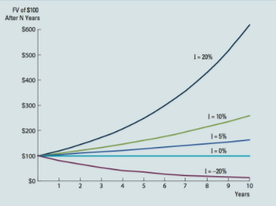
- Shown below is how a $100 investment grows (or declines) over time at different interest rates. Interest rates are normally positive, but the “growth” concept is broad enough to include negative rates. We developed the curves by solving the Equation with different values for N and I. The interest rate is a growth rate: If money is deposited and earns 5% per year, then your funds will grow by 5% per year. Note also that time value concepts can be applied to anything that grows—sales, population, earnings per share, or your future salary. Also, as noted before, the “growth rate” can be negative, as was sales growth for a number of auto companies in recent years.
2. when interest is earned on the interest earned in prior periods, we call it compound interest. If interest is earned only on the principal, we call it simple interest. The total interest earned with simple interest is equal to the principal multiplied by the interest rate times the number of periods: PV(I)(N). The future value is equal to the principal plus the interest: FV = PV + PV(I)(N). For example, suppose you deposit $100 for 3 years and earn simple interest at an annual rate of 5%. Your balance at the end of 3 years would be:
3. Notice that this is less than the $115.76 we calculated earlier using compound interest. Most applications in finance are based on compound interest, but you should be aware that simple interest is still specified in some legal documents.
Last modified: Tuesday, August 14, 2018, 8:41 AM