Reading: Lesson 1 - Investment Returns and Risk
6.1.A - Investment Returns and Risk
1. Investment Returns and Risk
- We start from the basic premise that investors like returns and dislike risk; this is called risk aversion. Therefore, people will invest in relatively risky assets only if they expect to receive relatively high returns—the higher the perceived risk, the higher the expected rate of return an investor will demand.
- With most investments, an individual or business spends money today with the expectation of earning even more money in the future. However, most investments are risky. Following are brief definitions of return and risk.
- The concept of return provides investors with a convenient way to express the financial performance of an investment. To illustrate, suppose you buy 10 shares of a stock for $1,000. The stock pays no dividends, but at the end of 1 year you sell the stock for $1,100. What is the return on your $1,000 investment? One way to express an investment’s return is in dollar terms:
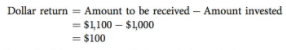
If instead at the end of the year you sell the stock for only $900, your dollar return will be −$100. Although expressing returns in dollars is easy, two problems arise: (1) To make a meaningful judgment about the return, you need to know the scale (size) of the investment; a $100 return on a $100 investment is a great return (assuming the investment is held for 1 year), but a $100 return on a $10,000 investment would be a poor return. (2) You also need to know the timing of the return; a $100 return on a $100 investment is a great return if it occurs after 1 year, but the same dollar return after 20 years is not very good. The solution to these scale and timing problems is to express investment results as rates of return, or percentage returns. For example, the rate of return on the 1-year stock investment, when $1,100 is received after 1 year, is 10%:
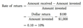
The rate of return calculation “standardizes” the dollar return by considering the annual return per unit of investment. Although this example has only one outflow and one inflow, the annualized rate of return can easily be calculated in situations where multiple cash flows occur over time by using time value of money concepts.
4. Risk is defined in Webster’s as “a hazard; a peril; exposure to loss or injury.” Thus, risk refers to the chance that some unfavorable event will occur. For an investment in financial assets or in new projects, the unfavorable event is ending up with a lower return than you expected. An asset’s risk can be analyzed in two ways: (1) on a stand-alone basis, where the asset is considered in isolation; and (2) on a portfolio basis, where the asset is held as one of a number of assets in a portfolio. Thus, an asset’s stand-alone risk is the risk an investor would face if she held only this one asset. Most assets are held in portfolios, but it is necessary to understand stand-alone risk in order to understand risk in a portfolio context.
2. Measuring Risk for Discrete Distributions
- Political and economic uncertainty affect stock market risk. For example, in the summer of 2011, the market fell sharply when Congress debated whether or not to raise the debt ceiling. Investors were unsure whether Congress would solve the crisis, come up with a temporary solution, or let the U.S. government default on Treasury securities and fall short on obligations to Social Security and Medicare. At the risk of oversimplification, these outcomes represented three distinct (or discrete) scenarios for the market, with each scenario having a very different market return.
- An event’s probability is defined as the chance that the event will occur. For example, a weather forecaster might state: “There is a 40% chance of rain today and a 60% chance that it will not rain.” If all possible events, or outcomes, are listed, and if a probability is assigned to each event, then the listing is called a probability distribution. (Keep in mind that the probabilities must sum to 1.0, or 100%
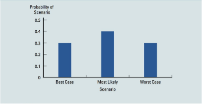
- Suppose an investor is facing a situation similar to the debt ceiling crisis and believes there are three possible outcomes for the market as a whole: (1) Best case, with a 30% probability; (2) Most Likely case, with a 40% probability; and (3) Worst case, with a 30% probability. The investor also believes the market would go up by 37% in the Best scenario, go up by 11% in the Most Likely scenario, and go down by 15% in the Worst scenario.
- The figure below shows the probability distribution for these three scenarios. Notice that the probabilities sum to 1.0 and that the possible returns are dispersed around the Most Likely scenario’s return.
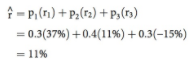
5. The rate-of-return probability distribution is shown in the “Inputs” section of the figure below; see Columns (1) and (2). This portion of the figure below is called a payoff matrix when the outcomes are cash flows or returns. If we multiply each possible outcome by its probability of occurrence and then sum these products, as in Column (3) of the figure below, the result is a weighted average of outcomes. The weights are the probabilities, and the weighted average is the expected rate of return, ^r, called “r-hat.”2 The expected rate of return is 11%, as shown in cell D66 in the figure below. The calculation for expected rate of return can also be expressed as an equation that does the same thing as the payoff matrix table:
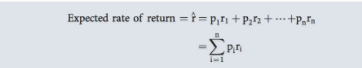

Here ri is the return if outcome i occurs, pi is the probability that outcome i occurs, and n is the number of possible outcomes. Thus, ^r is a weighted average of the possible outcomes (the ri values), with each outcome’s weight being its probability of occurrence. Using the data for from the figure above, we obtain the expected rate of return as follows:
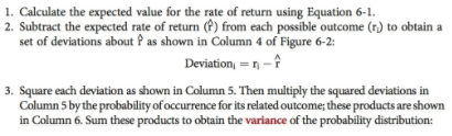
6. For simple distributions, it is easy to assess risk by looking at the dispersion of possible outcomes— a distribution with widely dispersed possible outcomes is riskier than one with narrowly dispersed outcomes. For example, we can look at Figure above and see that the possible returns are widely dispersed. But when there are many possible outcomes and we are comparing many different investments, it isn’t possible to assess risk simply by looking at the probability distribution—we need a quantitative measure of the tightness of the probability distribution. One such measure is the standard deviation, the symbol for which is σ, pronounced “sigma.” A large standard deviation means that possible outcomes are widely dispersed, whereas a small standard deviation means that outcomes are more tightly clustered around the expected value. To calculate the standard deviation, we proceed as shown in the figure below, taking the following steps:
![]()
![]()

The standard deviation provides an idea of how far above or below the expected value the actual value is likely to be. Using this procedure in the figure above, our hypothetical investor believes that the market return has a standard deviation of about 20%.
3. Risk in a Continuous Distribution
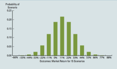
- Investors usually don’t estimate discrete outcomes in normal economic times but instead use the scenario approach during special situations, such as the debt ceiling crisis, the European bond crisis, oil supply threats, bank stress tests, and so on. Even in these situations, they would estimate more than 3 outcomes. For example, an investor might add more scenarios to our example; the figure below shows 15 scenarios for our original example.
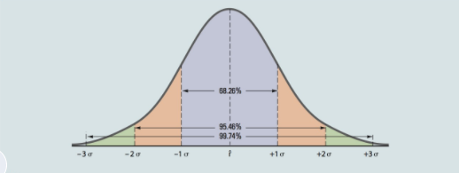
- We live in a complex world, with an infinite number of outcomes. But instead of adding more and more scenarios, most analysts turn to continuous distributions, with one of the most widely used being the normal distribution. With a normal distribution, the actual return will be within ±1 standard deviation of the expected return 68.26% of the time. Figure below illustrates this point, and it also shows the situation for ±2σ and ±3σ. For our 3-scenario example, ^r = 11% and σ = 20%. If returns come from a normal distribution with the same expected value and standard deviation rather than the discrete distribution, here would be a 68.26% probability that the actual return would be in the range of 11% ± 20%, or from −9% to 31%.
Last modified: Tuesday, August 14, 2018, 8:45 AM