Reading: Lesson 2 - Using Historical Data to Estimate Risk
6.2.A - Using Historical Data to Estimate Risk
1. Using Historical Data to Estimate Risk
- Suppose that a sample of returns over some past period is available. These past realized rates of return are denoted as −rt (“r bar t”), where t designates the time period. The average annual return over the last T periods is denoted as −r Avg:


The standard deviation of a sample of returns can then be estimated using this formula:


2. To illustrate these calculations, consider the following historical returns for a company:

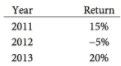
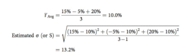

The average and standard deviation can also be calculated using Excel’s built-in functions, shown below using numerical data rather than cell ranges as inputs:
![]()
![]()
The historical standard deviation is often used as an estimate of future variability. Because past variability is often repeated, past variability may be a reasonably good estimate of future risk. However, it is usually incorrect to use −r Avg based on a past period as an estimate of ^r, the expected future return. For example, just because a stock had a 75% return in the past year, there is no reason to expect a 75% return this year.
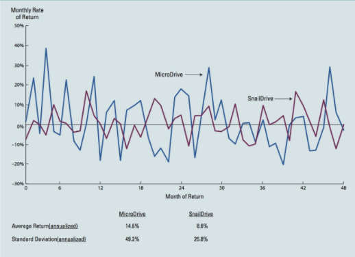
3. We could use the equations above to calculate the average return and standard deviation, but that would be quite tedious. Instead, we use Excel’s AVERAGE and STDEV functions and find that MicroDrive’s monthly average return was 1.22% and its monthly standard deviation was 14.19%. SnailDrive had an average monthly return of 0.72% and a standard deviation of 7.45%. These calculations confirm the visual evidence in the figure below: MicroDrive had greater stand-alone risk than SnailDrive.
4. We often use monthly data to estimate averages and standard deviations, but we normally present data in an annualized format. Multiply the monthly average return by 12 to get MicroDrive’s annualized average return of 1.22%(12) = 14.6%. As noted earlier, the past average return isn’t a good indicator of the future return. To annualize the standard deviation, multiply the monthly standard deviation by the square root of 12. MicroDrive’s annualized standard deviation was 14.19%( 12) = 49.2%. SnailDrive’s average annual return was 8.6% and its annualized standard deviation was 25.8%. Notice that MicroDrive had higher risk than SnailDrive (a standard deviation of 49.2% versus 25.8%) and a higher average return (14.6% versus 8.6%) during the past 48 months. However, a higher return for undertaking more risk isn’t guaranteed—if it were, then a riskier investment wouldn’t really by risky.


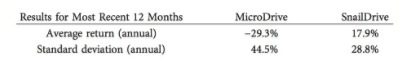
Even though MicroDrive’s standard deviation remained well above that of SnailDrive during the last 12 months of the sample period, MicroDrive experienced an annualized average loss of over 29% while SnailDrive gained almost 18%.6 MicroDrive’s stockholders certainly learned that higher risk doesn’t always lead to higher actual returns.
The Historic Trade-Off between Risk and Return
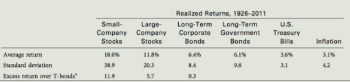
This historical trade-off between risk and return for different classes of investments. The assets that produced the highest average returns also had the highest standard deviations and the widest ranges of returns. For example, small-company stocks had the highest average annual return, but their standard deviation of returns also was the highest. In contrast, U.S. Treasury bills had the lowest standard deviation, but they also had the lowest average return. Note that a T-bill is riskless if you hold it until maturity, but if you invest in a rolling portfolio of T-bills and hold the portfolio for a number of years, then your investment income will vary depending on what happens to the level of interest rates in each year. You can be sure of the return you will earn on an individual T-bill, but you cannot be sure of the return you will earn on a portfolio of T-bills held over a number of years.
Last modified: Tuesday, August 14, 2018, 8:45 AM