Reading: Lesson 4 - The Capital Asset Pricing Model
6.4.A - The Capital Asset Pricing Model
1. Capital Asset Pricing Model (CAPM)
- We assume that investors are risk averse and demand a premium for bearing risk; that is, the higher the risk of a security, the higher its expected return must be to induce investors to buy it or to hold it. All risk except that related to broad market movements can, and presumably will, be diversified away. After all, why accept risk that can be eliminated easily? This implies that investors are primarily concerned with the risk of their portfolios rather than the risk of the individual securities in the portfolio. How, then, should the risk of an individual stock be measured?
- The Capital Asset Pricing Model (CAPM) provides one answer to that question. A stock might be quite risky if held by itself, but—because diversification eliminates about half of its risk—the stock’s relevant risk is its contribution to a well-diversified portfolio’s risk, which is much smaller than the stock’s stand-alone risk.
- A well-diversified portfolio has only market risk. Therefore, the CAPM defines the relevant risk of an individual stock as the amount of risk that the stock contributes to the market portfolio, which is a portfolio containing all stocks.12 In CAPM terminology, ρiM is the correlation between Stock i’s return and the market return, σi is the standard deviation of Stock i’s return, and σM is the standard deviation of the market’s return. The relevant measure of risk is called beta. The beta of Stock i, denoted by bi, is calculated as:
![]()
4. This formula shows that a stock with a high standard deviation, σi, will tend to have a high beta, which means that, other things held constant, the stock contributes a lot of risk to a well-diversified portfolio. This makes sense, because a stock with high stand-alone risk will tend to destabilize a portfolio. Note too that a stock with a high correlation with the market, ρiM, will also tend to have a large beta and hence be risky. This also makes sense, because a high correlation means that diversification is not helping much, with the stock performing well when the portfolio is also performing well, and the stock performing poorly when the portfolio is also performing poorly.
5. Suppose a stock has a beta of 1.4. What does that mean? To answer that question, we begin with an important fact: The beta of a portfolio, bp, is the weighted average of the betas of the stocks in the portfolio, with the weights equal to the same weights used to create the portfolio. This can be written as:

6. For example, suppose an investor owns a $100,000 portfolio consisting of $25,000 invested in each of four stocks; the stocks have betas of 0.6, 1.2, 1.2, and 1.4. The weight of each stock in the portfolio is $25,000/$100,000 = 25%. The portfolio’s beta will be bp = 1.1:
![]()
7. The second important fact is that the standard deviation of a well-diversified portfolio, σp, is approximately equal to the product of the portfolio’s beta and the market standard deviation:
![]()
The equation above shows that (1) a portfolio with a beta greater than 1 will have a bigger standard deviation than the market portfolio; (2) a portfolio with a beta equal to 1 will have the same standard deviation as the market; and (3) a portfolio with a beta less than 1 will have a smaller standard deviation than the market. For example, suppose the market standard deviation is 20%. Using the equation above, a well-diversified portfolio with a beta of 1.1 will have a standard deviation of 22%:
![]()
8. We can see the impact that each individual stock beta has on the risk of a well-diversified portfolio:

A well-diversified portfolio would have more than 4 stocks, but for the sake of simplicity suppose that the 4-stock portfolio in the previous example is well diversified. If that is the case, then the figure above shows how much risk each stock contributes to the portfolio.13 Out of the total 22% standard deviation of the portfolio, Stock 1 contributes w1b1σM = (25%)(0.6)(20%) = 3%. Stocks 2 and 3 have betas that are twice as big as Stock 1’s beta, so Stock’s 2 and 3 contribute twice as much risk as Stock 1. Stock 4 has the largest beta, and it contributes the most risk.
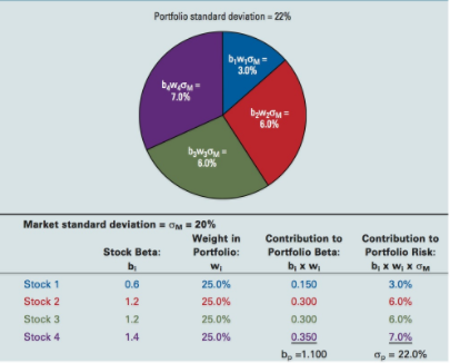
We demonstrate how to estimate beta in the next section, but here are some key points about beta. (1) Beta measures how much risk a stock contributes to a well-diversified portfolio. If all the stocks’ weights in a portfolio are equal, then a stock with a beta that is twice as big as another stock’s beta contributes twice as much risk. (2) The average of all stocks’ betas is equal to 1; the beta of the market also is equal to 1. Intuitively, this is because the market return is the average of all the stocks’ returns. (3) A stock with a beta greater than 1 contributes more risk to a portfolio than does the average stock, and a stock with a beta less than 1 contributes less risk to a portfolio than does the average stock. (4) Most stocks have betas that are between about 0.4 and 1.6.
2. Estimating Beta
- The CAPM is an ex ante model, which means that all of the variables represent before-the-fact, expected values. In particular, the beta coefficient used by investors should reflect the relationship between a stock’s expected return and the market’s expected return during some future period. However, people generally calculate betas using data from some past period and then assume that the stock’s risk will be the same in the future as it was in the past.
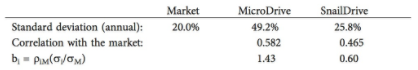
- Most analysts use 4 to 5 years of monthly data, although some use 52 weeks of weekly data. Using 4 years of monthly returns we can calculate the betas of MicroDrive and SnailDrive using the Beta Equation above:
3. The covariance between Stock i and the market, COViM, is defined as:
![]()
Calculate covariance by using another frequently used expression for calculating beta:
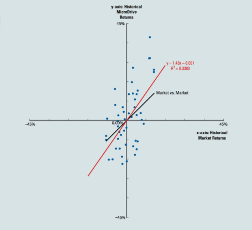
![]()
4. First, always keep in mind that beta cannot be observed, it can only be estimated. The R2 value shown in the chart measures the degree of dispersion about the regression line. Statistically speaking, it measures the percentage of the variance that is explained by the regression equation. An R2 of 1.0 indicates that all points lie exactly on the regression line and hence that all of the variations in the y-variable are explained by the x-variable. MicroDrive’s R2 is about 0.34, which is similar to the typical stock’s R2 of 0.32. This indicates that about 34% of the variance in MicroDrive’s returns is explained by the market return; in other words, much of MicroDrive’s volatility is due to factors other than market gyrations. If we had done a similar analysis for a portfolio of 40 randomly selected stocks, then the points would probably have been clustered tightly around the regression line and the R2 probably would have exceeded 0.90. Almost 100% of a well-diversified portfolio’s volatility is explained by the market.
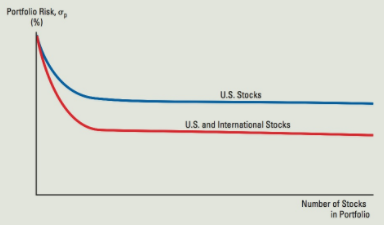
The Benefits of Diversifying Overseas
An investor can significantly reduce portfolio risk by holding a large number of stocks. Investors may be able to reduce risk even further by holding stocks from all around the world, because the returns on domestic and international stocks are not perfectly correlated.
3. The Relationship between Risk and Return in the Capital Asset Pricing Model
- The CAPM assumes that the marginal investors (i.e., the investors with enough cash to move market prices) hold well-diversified portfolios. Therefore, beta is the proper measure of a stock’s relevant risk. However, we need to quantify how risk affects required returns: For a given level of risk as measured by beta, what rate of expected return do investors require to compensate them for bearing that risk? To begin, we define the following terms.
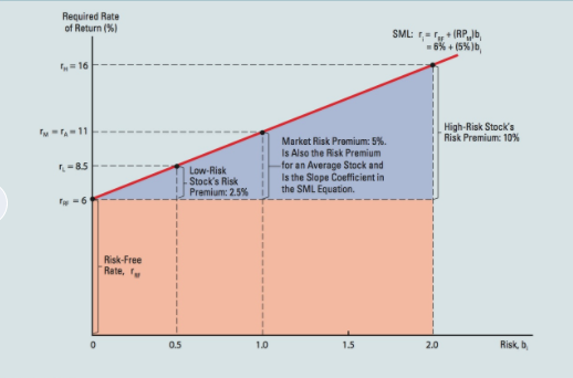
2. The CAPM’s Security Market Line (SML) formalizes this general concept by showing that a stock’s risk premium is equal to the product of the stock’s beta and the market risk premium:
Notice that a stock’s required return begins with the risk-free rate. To induce an investor to take on a risky investment, the investor will need a return that is at least as big as the risk-free rate. The yield on long-term Treasury bonds is often used to measure the risk-free rate.
3. The market risk premium, RPM, is the extra rate of return that investors require to invest in the stock market rather than purchase risk-free securities. The size of the market risk premium depends on the degree of risk aversion that investors have on average. When investors are very risk averse, the market risk premium is high; when investors are less concerned about risk, the market risk premium is low. For example, suppose that investors (on average) need an extra return of 5% before they will take on the stock market’s risk. If Treasury bonds yield rRF = 6%, then the required return on the market, rM, is 11%:
![]()
4. The CAPM shows that the risk premium for an individual stock, RPi, is equal to the product of the stock’s beta and the market risk premium:
![]()
For example, consider a low-risk stock with bL = 0.5. If the market risk premium is 5%, then the risk premium for the stock (RPL) is 2.5%:
![]()
Using the SML, the required return for our illustrative low-risk stock is then found as follows:
![]()
If a high-risk stock has bH = 2.0, then its required rate of return is 16%:
![]()
An average stock, with bA = 1.0, has a required return of 11%, the same as the market return:
![]()
1. Required rates of return are shown on the vertical axis, while risk as measured by beta is shown on the horizontal axis. This graph is quite different from the regression line shown in the figure above, where the returns on individual stocks were plotted on the vertical axis and returns on the market index were shown on the horizontal axis. For the SML in Figure above, the slope of the regression line from an analysis such as that conducted in the figure above is plotted as beta on the horizontal axis of the figure above.
2. Riskless securities have bi = 0; therefore, rRF appears as the vertical axis intercept in the figure above. If we could construct a portfolio that had a beta of zero, then it would have a required return equal to the risk-free rate.
3. The slope of the SML (5% in the figure above) reflects the degree of risk aversion in the economy: The greater the average investor’s aversion to risk, then (a) the steeper the slope of the line, (b) the greater the risk premium for all stocks, and (c) the higher the required rate of return on all stocks.
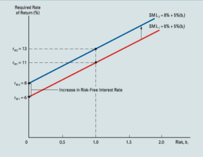
4. The Impact on Required Return Due to Changes in the Risk-Free Rate, Risk Aversion, and Beta
- The required return depends on the risk-free rate, the market risk premium, and the stock’s beta. Suppose that some combination of an increase in real interest rates and in anticipated inflation causes the risk-free interest rate to increase from 6% to 8%. Such a change is shown in the figure below. A key point to note is that a change in rRF will not necessarily cause a change in the market risk premium. Thus, as rRF changes, so will the required return on the market, and this will, other things held constant, keep the market risk premium stable.17 Notice that, under the CAPM, the increase in rRF leads to an identical increase in the rate of return on all assets, because the same risk-free rate is built into the required rate of return on all assets. For example, the required rate of return on the market (and the average stock), rM, increases from 11% to 13%. Other risky securities’ returns also rise by 2 percentage points.
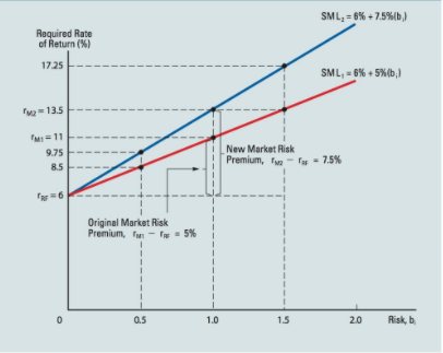
2. The slope of the Security Market Line reflects the extent to which investors are averse to risk: The steeper the slope of the line, the greater the average investor’s aversion to risk. Suppose all investors were indifferent to risk—that is, suppose they were not risk averse. If rRF were 6%, then risky assets would also provide an expected return of 6%, because if there were no risk aversion then there would be no risk premium, and the SML would be plotted as a horizontal line. As risk aversion increases, so does the risk premium, and this causes the slope of the SML to become steeper.
3. The figure below illustrates an increase in risk aversion. The market risk premium rises from 5% to 7.5%, causing rM to rise from rM1 = 11% to rM2 = 13.5%. The returns on other risky assets also rise, and the effect of this shift in risk aversion is greater for riskier securities. For example, the required return on a stock with bi = 0.5 increases by only 1.25 percentage points, from 8.5% to 9.75%; that on a stock with bi = 1.0 increases by 2.5 percentage points, from 11.0% to 13.5%; and that on a stock with bi = 1.5 increases by 3.75 percentage points, from 13.5% to 17.25%.
4. Given risk aversion and a positively sloped SML as in the figure above, the higher a stock’s beta, the higher its required rate of return. As we shall see later in the book, a firm can influence its beta through changes in the composition of its assets and also through its use of debt: Acquiring riskier assets will increase beta, as will a change in capital structure that calls for a higher debt ratio. A company’s beta can also change as a result of external factors such as increased competition in its industry, the expiration of basic patents, and the like. When such changes lead to a higher or lower beta, the required rate of return will also change.
5. Portfolio Returns and Portfolio Performance Evaluation
- The expected return on a portfolio, ^rp, is the weighted average of the expected returns on the individual assets in the portfolio. Suppose there are n stocks in the portfolio and the expected return on Stock i is ^r i. The expected return on the portfolio is:
![]()
2. The required return on a portfolio, rp, is the weighted average of the required returns on the individual assets in the portfolio:
![]()
We can also express the required return on a portfolio in terms of the portfolio’s beta:
![]()
This is particularly helpful when evaluating portfolio managers. For example, suppose the stock market has a return for the year of 9% and a particular mutual fund has a 10% return. Did the portfolio manager do a good job or not? The answer depends on how much risk the fund has. If the fund’s beta is 2, then the fund should have had a much higher return than the market, which means the manager did not do well. The key is to evaluate the portfolio manager’s return against the return the manager should have made given the risk of the investments.
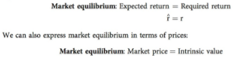
6. Required Returns versus Expected Returns: Market Equilibrium
- We have explained that managers should seek to maximize the value of their firms’ stocks. We also have emphasized the difference between the market price and intrinsic value. Intrinsic value incorporates all relevant available information about expected cash flows and risk. This includes information about the company, the economic environment, and the political environment. In contrast to intrinsic value, market prices are based on investors’ selection and interpretation of information. To the extent that investors don’t select all relevant information and don’t interpret it correctly, market prices can deviate from intrinsic values. The figure below illustrates this relationship between market prices and intrinsic value.
- When market prices deviate from their intrinsic values, astute investors have profitable opportunities. For example, recall that the value of a bond is the present value of its cash flows when discounted at the bond’s required return, which reflects the bond’s risk. This is the intrinsic value of the bond because it incorporates all relevant available information. Notice that the intrinsic value is “fair” in the sense that it incorporates the bond’s risk and investors’ required returns for bearing the risk.
- What would happen if a bond’s market price were lower than its intrinsic value? In this situation, an investor could purchase the bond and receive a rate of return in excess of the required return. In other words, the investor would get more compensation than justified by the bond’s risk. If all investors felt this way, then demand for the bond would soar as investors tried to purchase it, driving the bond’s price up. But recall that as the price of a bond goes up, its yield goes down. This means that an increase in price would reduce the subsequent return for an investor purchasing (or holding) the bond at the new price. It seems reasonable to expect that investors’ actions would continue to drive the price up until the expected return on the bond equaled its required return. After that point, the bond would provide just enough return to compensate its owner for the bond’s risk.
- If the bond’s price were too high compared to its intrinsic value, then investors would sell the bond, causing its price to fall and its yield to increase until its expected return equaled its required return. A stock’s future cash flows aren’t as predictable as a bond’s, but we show in the next chapter that a stock’s intrinsic value is the present value of its expected future cash flows, just as a bond’s intrinsic value is the present value of its cash flows. If the price of a stock is lower than its intrinsic value, then an investor would receive an expected return greater than the return required as compensation for risk. The same market forces we described for a mispriced bond would drive the mispriced stock’s price up. If this process continues until its expected return equals it required return, then we say that there is market equilibrium:
Last modified: Tuesday, August 14, 2018, 8:45 AM