Reading: Lesson 6 - Managerial Issues and the Cost of Capital
8.6.A - Managerial Issues and the Cost of Capital
1. Privately Owned Firms and Small Businesses
- When we estimated the rate of return required by public stockholders, we use stock returns to estimate beta as an input for the CAPM approach and stock prices as input data for the DCF method. But how can one measure the cost of equity for a firm whose stock is not traded? Most analysts begin by identifying one or more publicly traded firms that are in the same industry and that are approximately the same size as the privately owned firm.16 The analyst then estimates the betas for these publicly traded firms and uses their average beta as an estimate of the beta of the privately owned firm.
- we know that a company’s cost of debt is above the risk-free rate due to the default risk premium. We also know that a company’s cost of stock should be greater than its cost of debt because equity is riskier than debt. Therefore, some analysts use a subjective, ad hoc procedure to estimate a firm’s cost of common equity: They simply add a judgmental risk premium of 3% to 5% to the cost of debt. In this approach

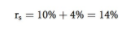
For example, consider a privately held company with a 10% cost of debt. Using 4% as the judgmental risk premium (because it is the mid-point of the 3%–5% range), the estimated cost of equity is 14%:
The stock of a privately held firm is less liquid than that of a publicly held firm. Investors require a liquidity premium on thinly traded bonds. Therefore, many analysts make an ad hoc adjustment to reflect this lack of liquidity by adding 1 to 3 percentage points to the firm’s cost of equity. This rule of thumb is not theoretically satisfying because we don’t know exactly how large the liquidity premium should be, but it is logical and is also a common practice.
Suppose a privately held firm is concerned that its current capital structure weights are appropriate. The first step for a publicly traded company would be to estimate the capital structure weights based on current market values. However, a privately held firm can’t directly observe its market value, so it can’t directly observe its market value weights.
To resolve this problem, many analysts begin by making a trial guess as to the value of the firm’s equity. The analysts then use this estimated value of equity to estimate the cost of capital, next use the cost of capital to estimate the value of the firm, and finally complete the circle by using the estimated value of the firm to estimate the value of its equity. If this newly estimated equity value is different from their trial guess, analysts repeat the process but start the iteration with the newly estimated equity value as the trial value of equity. After several iterations, the trial value of equity and the resulting estimated equity value usually converge. Although somewhat tedious, this process provides consistent estimates of the weights, the cost of capital, and the value of the firm.
2. Managerial Issues and the Cost of Capital
- Four factors are beyond managerial control: (1) interest rates, (2) credit crises, (3) the market risk premium, and (4) tax rates.
- Interest rates in the economy affect the costs of both debt and equity, but they are beyond a manager’s control. Even the Fed can’t control interest rates indefinitely. For example, interest rates are heavily influenced by inflation, and when inflation hit historic highs in the early 1980s, interest rates followed. Rates trended mostly down for 25 years through the recession accompanying the 2008 financial crisis. Strong actions by the federal government in the spring of 2009 brought rates even lower, which contributed to the official ending of the recession in June 2009. These actions encouraged investment, and there is little doubt that they will eventually lead to stronger growth. However, many observers fear that the government’s actions will also reignite long-run inflation, which would lead to higher interest rates.
- Although rare, sometimes credit markets are so disrupted that it is virtually impossible for a firm to raise capital at reasonable rates. This happened in 2008 and 2009, before the U.S. Treasury and the Federal Reserve intervened to open up the capital markets. During such times, firms tend to cut back on growth plans; if they must raise capital, its cost can be extraordinarily high.
- Investors’ aversion to risk determines the market risk premium. Individual firms have no control over the RPM, which affects the cost of equity and thus the WACC.
- Tax rates, which are influenced by the president and set by Congress, have an important effect on the cost of capital. They are used when we calculate the after-tax cost of debt for use in the WACC. In addition, the lower tax rate on dividends and capital gains than on interest income favors financing with stock rather than bonds.
- A firm can affect its cost of capital through (1) its capital structure policy, (2) its dividend policy, and (3) its investment (capital budgeting) policy.
- we assume the firm has a given target capital structure, and we use weights based on that target to calculate its WACC. However, a firm can change its capital structure, and such a change can affect the cost of capital. For example, the after-tax cost of debt is lower than the cost of equity, so if the firm decides to use more debt and less common equity, then this increase in debt will tend to lower the WACC. However, an increased use of debt will increase the risk of debt and the equity, offsetting to some extent the effect due to a greater weighting of debt.
- The percentage of earnings paid out in dividends may affect a stock’s required rate of return, rs. Also, if the payout ratio is so high that the firm must issue new stock to fund its capital budget, then the resulting flotation costs will also affect the WACC.
- When we estimate the cost of capital, we use as the starting point the required rates of return on the firm’s outstanding stocks and bonds, which reflect the risks inherent in the existing assets. Therefore, we are implicitly assuming that new capital will be invested in assets with the same degree of risk as existing assets. This assumption is generally correct, because most firms invest in assets similar to those they currently use. However, the equal risk assumption is incorrect if a firm dramatically changes its investment policy. For example, if a company invests in an entirely new line of business, then its marginal cost of capital should reflect the risk of that new business. For example, we can see with hindsight that GE’s huge investments in the TV and movie businesses, as well as its investment in mortgages, increased its risk and thus its cost of capital.
3. Adjusting the Cost of Capital for Risk
- As we have calculated it, the weighted average cost of capital reflects the average risk and overall capital structure of the entire firm. No adjustments are needed when using the WACC as the discount rate when estimating the value of a company by discounting its cash flows. However, adjustments for risk are often needed when evaluating a division or project. For example, what if a firm has divisions in several business lines that differ in risk? Or what if a company is considering a project that is much riskier than its typical project? It is not logical to use the overall cost of capital to discount divisional or project-specific cash flows that don’t have the same risk as the company’s average cash flows. The following sections explain how to adjust the cost of capital for divisions and for specific projects.
- Consider Starlight Sandwich Shops, a company with two divisions—a bakery operation and a chain of cafes. The bakery division is low-risk and has a 10% WACC. The cafe division is riskier and has a 14% WACC. Each division is approximately the same size, so Starlight’s overall cost of capital is 12%. The bakery manager has a project with an 11% expected rate of return, and the cafe division manager has a project with a 13% expected return. Should these projects be accepted or rejected? Starlight will create value if it accepts the bakery’s project, because its rate of return is greater than its cost of capital (11% > 10%), but the cafe project’s rate of return is less than its cost of capital (13% < 14%), so it should reject that project. However, if management simply compared the two projects’ returns with Starlight’s 12% overall cost of capital, then the bakery’s value-adding project would be rejected while the cafe’s value-destroying project would be accepted.
- Many firms use the CAPM to estimate the cost of capital for specific divisions. To begin, recall that the Security Market Line (SML) equation expresses the risk–return relationship as follows:

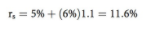
As an example, consider the case of Huron Steel Company, an integrated steel producer operating in the Great Lakes region. For simplicity, assume that Huron has only one division and uses only equity capital, so its cost of equity is also its corporate cost of capital, or WACC. Huron’s beta = b = 1.1, rRF = 5%, and RPM = 6%. Thus, Huron’s cost of equity (and WACC) is 11.6%:
This suggests that investors should be willing to give Huron money to invest in new, average-risk projects if the company expects to earn 11.6% or more on this money. By “average risk” we mean projects having risk similar to the firm’s existing division. Now suppose Huron creates a new transportation division consisting of a fleet of barges to haul iron ore, and suppose barge operations typically have betas of 1.5 rather than 1.1. The barge division, with b = 1.5, has a 14.0% cost of capital:

On the other hand, if Huron adds a low-risk division, such as a new distribution center with a beta of only 0.5, then that division’s cost of capital would be 8%:

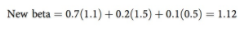
A firm itself may be regarded as a “portfolio of assets,” and because the beta of a portfolio is a weighted average of the betas of its individual assets, adding the barge and distribution center divisions will change Huron’s overall beta. The exact value of the new corporate beta would depend on the size of the investments in the new divisions relative to Huron’s original steel operations. If 70% of Huron’s total value ends up in the steel division, 20% in the barge division, and 10% in the distribution center, then its new corporate beta would be calculated as follows:
Thus, investors in Huron’s stock would require a return of

Even though investors require an overall return of 11.72%, they should expect a rate of return on projects in each division at least as high as the division’s required return based on the SML. In particular, they should expect a return of at least 11.6% from the steel division, 14.0% from the barge division, and 8.0% from the distribution center. Our example suggests a level of precision that is much higher than firms can obtain in the real world. Still, managers should be aware of this example’s logic, and they should strive to measure the required inputs as accurately as possible.
In Unit 6 we discussed the estimation of betas for stocks and indicated how difficult it is to measure beta precisely. Estimating divisional betas is much more difficult, primarily because divisions do not have their own publicly traded stock. Therefore, we must estimate the beta that the division would have if it were an independent, publicly traded company. Two approaches can be used to estimate divisional betas: the pure play method and the accounting beta method.
The Pure Play Method. In the pure play method, the company tries to find the betas of several publicly held specialized companies in the same line of business as the division being evaluated, and it then averages those betas to determine the cost of capital for its own division. For example, suppose Huron found three companies devoted exclusively to operating barges, and suppose that Huron’s management believes its barge division would be subject to the same risks as those firms. Then Huron could use the average beta of those firms as an estimate of its barge division’s beta.
As noted above, it may be impossible to find specialized publicly traded firms suitable for the pure play approach. If that is the case, we may be able to use the accounting beta method. Betas are normally found by regressing the returns of a particular company’s stock against returns on a stock market index. However, we could run a regression of the division’s accounting return on assets against the average return on assets for a large sample of companies, such as those included in the S&P 500. Betas determined in this way (that is, by using accounting data rather than stock market data) are called accounting betas.
First, although it is intuitively clear that riskier projects have a higher cost of capital, it is difficult to measure projects’ relative risks. Also, note that three separate and distinct types of risk can be identified.
1. Stand-alone risk, which is the variability of the project’s expected returns.
2. Corporate, or within-firm, risk, which is the variability the project contributes to the corporation’s returns, giving consideration to the fact that the project represents only one asset of the firm’s portfolio of assets and so some of its risk will be diversified away.
3. Market, or beta, risk, which is the risk of the project as seen by a well-diversified stockholder who owns many different stocks. A project’s market risk is measured by its effect on the firm’s overall beta coefficient.Taking on a project with a high degree of either stand-alone or corporate risk will not necessarily increase the corporate beta. However, if the project has highly uncertain returns and if those returns are highly correlated with returns on the firm’s other assets and with most other assets in the economy, then the project will have a high degree of all types of risk.
Of the three measures, market risk is theoretically the most relevant because of its direct effect on stock prices. Unfortunately, the market risk for a project is also the most difficult to estimate. In practice, most decision makers consider all three risk measures in a subjective manner.
The first step is to determine the divisional cost of capital before grouping divisional projects into subjective risk categories. Then, using the divisional WACC as a starting point, risk-adjusted costs of capital are developed for each category. For example, a firm might establish three risk classes—high, average, and low—and then assign average- risk projects the divisional cost of capital, higher-risk projects an above-average cost, and lower-risk projects a below-average cost. Thus, if a division’s WACC were 10%, its managers might use 10% to evaluate average-risk projects in the division, 12% for high-risk projects, and 8% for low-risk projects. Although this approach is better than ignoring project risk, these adjustments are necessarily subjective and somewhat arbitrary. Unfortunately, given the data, there is no completely satisfactory way to specify exactly how much higher or lower we should go in setting risk-adjusted costs of capital.
4. Four Mistakes to Avoid
- We often see managers and students make the following mistakes when estimating the cost of capital. Although we have discussed these errors previously at separate places in the chapter, they are worth repeating here.
1. Never base the cost of debt on the coupon rate on a firm’s existing debt. The cost of debt must be based on the interest rate the firm would pay if it issued new debt today.
2. When estimating the market risk premium for the CAPM method, never use the historical average return on stocks in conjunction with the current return on T-bonds. The historical average return on bonds should be subtracted from the past average return on stocks to calculate the historical market risk premium. On the other hand, it is appropriate to subtract today’s yield on T-bonds from an estimate of the expected future return on stocks to obtain the forward-looking market risk premium. A case can be made for using either the historical or the current risk premium, but it would be wrong to take the historical rate of return on stocks, subtract from it the current rate on T-bonds, and then use the difference as the market risk premium.
3. Never use the current book value capital structure to obtain the weights when estimating the WACC. Your first choice should be to use the firm’s target capital structure for the weights. However, if you are an outside analyst and do not know the target weights, it would probably be best to estimate weights based on the current market values of the capital components. If the company’s debt is not publicly traded, then it is reasonable to use the book value of debt to estimate the weights because book and market values of debt, especially short-term debt, are usually close to one another. However, stocks’ market values in recent years have generally been at least 2–3 times their book values, so using book values for equity could lead to serious errors. The bottom line: If you don’t know the target weights then use the market value, not the book value, of equity when calculating the WACC.
4. Always remember that capital components are funds that come from investors. If it’s not from an investor, then it’s not a capital component. Sometimes the argument is made that accounts payable and accruals should be included in the calculation of the WACC. However, these funds are not provided by investors, but instead, they arise from operating relationships with suppliers and employees. As such, the impact of accounts payable and accruals is incorporated into the calculations of free cash flows and project cash flows. Therefore, accounts payable and accruals should not be included as capital components when we calculate the WACC.
Last modified: Tuesday, August 14, 2018, 8:50 AM