Reading: Lesson 4 - Relevant Cash Flows, Project Expansion, & Capital Budgeting Risk Analysis
9.4.A - Relevant Cash Flows, Project Expansion, & Capital Budgeting Risk Analysis
1. Identifying Relevant Cash Flows
- The most important—and difficult—step in capital budgeting is estimating a proposal’s relevant project cash flows, which are the differences between the cash flows the firm will have if it implements the project versus the cash flows it will have if it rejects the project. These are called incremental cash flows:

Estimating incremental cash flows might sound easy, but there are many potential pitfalls. In this section, we identify the key concepts that will help you avoid these pitfalls and then apply the concepts to an actual project to illustrate their application to cash flow estimation.
Free cash flow is cash flow that is available for distribution to investors, making free cash flow the basis of a firm’s value. It is common in the practice of finance to speak of a firm’s free cash flow and a project’s cash flow (or net cash flow), but these are based on the same concepts. In fact, a project’s cash flow is identical to the project’s free cash flow, and a firm’s total net cash flow from all projects is equal to the firm’s free cash flow. We will follow the typical convention and refer to a project’s free cash flow simply as project cash flow, but keep in mind that the two concepts are identical.
Because net income is not equal to the cash flow available for distribution to investors, in the last chapter we discounted net cash flows, not accounting income, to find projects’ NPVs. For capital budgeting purposes it is the project’s net cash flow, not its accounting income, which is relevant. Therefore, when analyzing a proposed capital budgeting project, disregard the project’s net income and focus exclusively on its net cash flow. Be especially alert to the following differences between cash flow and accounting income.
Most projects require assets, and asset purchases represent negative cash flows. Even though the acquisition of assets results in a cash outflow, accountants do not show the purchase of fixed assets as a deduction from accounting income. Instead, they deduct a depreciation expense each year throughout the life of the asset. Depreciation shelters income from taxation, and this has an impact on cash flow, but depreciation itself is not a cash flow. Therefore, depreciation must be added back when estimating a project’s operating cash flow.
Depreciation is the most common noncash charge, but there are many other noncash charges that might appear on a company’s financial statements. Just as with depreciation, all other noncash charges should be added back when calculating a project’s net cash flow.
Normally, additional inventories are required to support a new operation, and expanded sales tie up additional funds in accounts receivable. However, payables and accruals increase as a result of the expansion, and this reduces the cash needed to finance inventories and receivables. The difference between the required increase in operating current assets and the increase in operating current liabilities is the change in net operating working capital. If this change is positive, as it generally is for expansion projects, then additional financing—beyond the cost of the fixed assets— will be needed.
Toward the end of a project’s life, inventories will be used but not replaced, and receivables will be collected without corresponding replacements. As these changes occur the firm will receive cash inflows; as a result, the investment in net operating working capital will be returned by the end of the project’s life.
Interest is a cash expense, so at first blush it would seem that interest on any debt used to finance a project should be deducted when we estimate the project’s net cash flows. However, this is not correct. Recall that we discount a project’s cash flows by its risk-adjusted cost of capital, which is a weighted average (WACC) of the costs of debt, preferred stock, and common equity, adjusted for the project’s risk and debt capacity. This project cost of capital is the rate of return necessary to satisfy all of the firm’s investors, including stockholders and debtholders. A common mistake made by many students and financial managers is to subtract interest payments when estimating a project’s cash flows. This is a mistake because the cost of debt is already embedded in the cost of capital, so subtracting interest payments from the project’s cash flows would amount to double-counting interest costs. Therefore, you should not subtract interest expenses when finding a project’s cash flows.
In theory, in capital budgeting analyses we should discount cash flows based on the exact moment when they occur. Therefore, one could argue that daily cash flows would be better than annual flows. However, it would be costly to estimate daily cash flows and laborious to analyze them. In general the analysis would be no better than one using annual flows because we simply can’t make accurate forecasts of daily cash flows more than a couple of months into the future. Therefore, it is generally appropriate to assume that all cash flows occur at the end of the various years. For projects with highly predictable cash flows, such as constructing a building and then leasing it on a long-term basis (with monthly payments) to a financially sound tenant, we would analyze the project using monthly periods.
Two types of projects can be distinguished: (1) expansion projects, in which the firm makes an investment in, for example, a new Home Depot store in Seattle; and (2) replacement projects, in which the firm replaces existing assets, generally to reduce costs. In expansion projects, the cash expenditures on buildings, equipment, and required working capital are obviously incremental, as are the sales revenues and operating costs associated with the project. The incremental costs associated with replacement projects are not so obvious. For example, Home Depot might replace some of its delivery trucks to reduce fuel and maintenance expenses. Replacement analysis is complicated by the fact that most of the relevant cash flows are the cash flow differences between the existing project and the replacement project. For example, the fuel bill for a more efficient new truck might be $10,000 per year versus $15,000 for the old truck, and the $5,000 fuel savings would be an incremental cash flow associated with the replacement decision.
A sunk cost is an outlay related to the project that was incurred in the past and that cannot be recovered in the future regardless of whether or not the project is accepted. Therefore, sunk costs are not incremental costs and thus are not relevant in a capital budgeting analysis.
To illustrate, suppose Home Depot spent $2 million to investigate sites for a potential new store in a given area. That $2 million is a sunk cost—the money is gone, and it won’t come back regardless of whether or not a new store is built. Therefore, the $2 million should not be included in a capital budgeting decision. Improper treatment of sunk costs can lead to bad decisions. For example, suppose Home Depot completed the analysis for a new store and found that it must spend an additional (or incremental) $17 million to build and supply the store, on top of the $2 million already spent on the site study. Suppose the present value of future cash flows is $18 million. Should the project be accepted? If the sunk costs are mistakenly included, the NPV is −$2 million + (−$17 million) + $18 million = −$1 million and the project would be rejected. However, that would be a bad decision. The real issue is whether the incremental $17 million would result in enough incremental cash flow to produce a positive NPV. If the $2 million sunk cost were disregarded, as it should be, then the NPV on an incremental basis would be a positive $1 million.
Another conceptual issue relates to opportunity costs related to assets the firm already owns. Continuing our example, suppose Home Depot (HD) owns land with a current market value of $2 million that can be used for the new store if it decides to build the store. If HD goes forward with the project, only another $15 million will be required, not the full $17 million, because it will not need to buy the required land. Does this mean that HD should use the $15 million incremental cost as the cost of the new store? The answer is definitely “no.” If the new store is not built, then HD could sell the land and receive a cash flow of $2 million. This $2 million is an opportunity cost—it is cash that HD would not receive if the land is used for the new store. Therefore, the $2 million must be charged to the new project, and failing to do so would cause the new project’s calculated NPV to be too high.
Another conceptual issue relates to externalities, which are the effects of a project on other parts of the firm or on the environment. As explained in what follows, there are three types of externalities: negative within-firm externalities, positive within-firm externalities, and environmental externalities.
If a retailer like Home Depot opens a new store that is close to its existing stores, then the new store might attract customers who would otherwise buy from the existing stores, reducing the old stores’ cash flows. Therefore, the new store’s incremental cash flow must be reduced by the amount of the cash flow lost by its other units. This type of externality is called cannibalization, because the new business eats into the company’s existing business. Many businesses are subject to cannibalization. For example, each new iPod model cannibalizes existing models. Those lost cash flows should be considered, and that means charging them as a cost when analyzing new products.
Dealing properly with negative externalities requires careful thinking. If Apple decided not to come out with a new model of iPod because of cannibalization, another company might come out with a similar new model, causing Apple to lose sales on existing models.
As we noted earlier, cannibalization occurs when a new product competes with an old one. However, a new project can also be complementary to an old one, in which case cash flows in the old operation will be increased when the new one is introduced. For example, Apple’s iPod was a profitable product, but when Apple considered an investment in its music store it realized that the store would boost sales of iPods. So, even if an analysis of the proposed music store indicated a negative NPV, the analysis would not be complete unless the incremental cash flows that would occur in the iPod division were credited to the music store. Consideration of positive externalities often changes a project’s NPV from negative to positive.
The most common type of negative externality is a project’s impact on the environment. Government rules and regulations constrain what companies can do, but firms have some flexibility in dealing with environmental issues. For example, suppose a manufacturer is studying a proposed new plant. The company could meet current environmental regulations at a cost of $1 million, but the plant would still emit fumes that would cause some bad will in its neighborhood. Those ill feelings would not show up in the cash flow analysis, but they should be considered. Perhaps a relatively small additional expenditure would reduce the emissions substantially, make the plant look good relative to other plants in the area, and provide goodwill that in the future would help the firm’s sales and its negotiations with governmental agencies.
Of course, all firms’ profits ultimately depend on the Earth remaining healthy, so companies have some incentive to do things that protect the environment even though those actions are not currently required. However, if one firm decides to take actions that are good for the environment but quite costly, then it must either raise its prices or suffer a decline in earnings. If its competitors decide to get by with less costly but environmen- tally unfriendly processes, they can price their products lower and make more money. Of course, the more environmentally friendly companies can advertise their environmental efforts, and this might—or might not—offset their higher costs. All this illustrates why government regulations are often necessary. Finance, politics, and the environment are all interconnected.
2. Analysis of an Expansion Project
- Earlier, we worked with the cash flows associated with one of Guyton Products Company’s expansion projects. Recall that Project L is the application of a radically new liquid nanocoating technology to a new type of solar water heater module, which will be manufactured under a 4-year license from a university. In this section we show how these cash flows are estimated (we only show estimates for Project L in the chapter, but we also show estimates GPC’s other project, Project S. It’s not clear how well the water heater will work, how strong demand for it will be, how long it will be before the product becomes obsolete, or whether the license can be renewed after the initial 4 years. Still, the water heater has the potential for being profitable, though it could also fail miserably. GPC is a relatively large company and this is one of many projects, so a failure would not bankrupt the firm but would hurt profits and the stock’s price.
- We used Excel to do the analysis. We could have used a calculator and paper, but Excel is much easier when dealing with capital budgeting problems. You don’t need to know Excel to understand our discussion, but if you plan to work in finance—or, really, in any business field—you must know how to use Excel, so we recommend that you open the Excel Tool Kit for this chapter and scroll through it as the textbook explains the analysis.
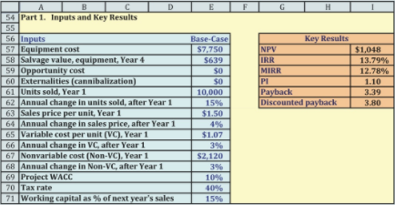
- The Figure below shows the Part 1 of the Excel model used in this analysis. The base-case inputs are in the blue section. For example, the cost of required equipment to manufacture the water heaters is $7,750 and is shown in the blue input section. (All dollar values in the Figure below and in our discussion here are reported in thousands, so the equipment actually costs $7,750,000.) The actual number-crunching takes place in Part 2 of the model, shown in the other Figure below. Part 2 takes the inputs from the blue section of Figure below and generates the project’s cash flows. Part 2 of the model also performs calculations of the project performance measures discussed in Chapter 10 and then reports those results in the orange section of the Figure below. This structure allows you (or your manager) to change and input and instantly see the impact on the reported performance measures.
3. Cash Flow Projections: Intermediate Calculations
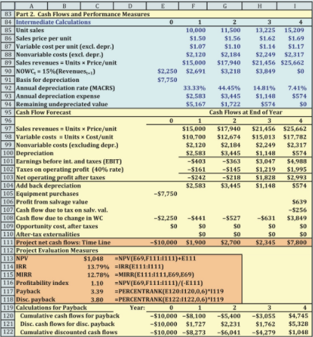
- The Figure below shows Part 2 of the model. When setting up Excel models, we prefer to have more rows but shorter formulas. So instead of having very complicated formulas in the section for cash flow forecasts, we put intermediate calculations in a separate section. The blue section of the Figure below shows these intermediate calculations for the GPC project, as we explain in the following sections.
- Rows 85–88 show annual unit sales, unit sale prices, unit variable costs, and nonvariable costs. These values are all projected to grow at the rates assumed in Part 1 of the model in Figure above. If you ignore growth in prices and costs when estimating cash flows, you are likely to underestimate a project’s value because the project’s weighted average cost of capital (WACC) includes the impact of inflation. In other words, the estimated cash flows will be too low relative to the WACC, so the estimated net present value (NPV) also will be too low relative to the true NPV. To see that the WACC includes inflation, recall that the cost of debt includes an inflation premium. Also, the capital asset pricing model defines the cost of equity as the sum of the risk-free rate and a risk premium. Like the cost of debt, the risk-free rate also has an inflation premium. Therefore, if the WACC includes the impact of inflation, the estimated cash flows must also include inflation. It is theoretically possible to ignore inflation when estimating the cash flows but adjust the WACC so that it, too, doesn’t incorporate inflation, but we have never seen this accomplished correctly in practice. Therefore, you should always include growth rates in prices and costs when estimating cash flows.
Virtually all projects require working capital, and this one is no exception. For example, raw materials must be purchased and replenished each year as they are used. In Part 1 (Figure above) we assume that GPC must have an amount of net operating working capital on hand equal to 15% of the upcoming year’s sales. For example, in Year 0, GPC must have 15%($15,000) = $2,250 in working capital on hand. As sales grow, so does the required working capital. Rows 89–90 show the annual sales revenues (the product of units sold and sales price) and the required working capital.
Rows 91–94 report intermediate calculations related to depreciation, beginning with the depreciation basis, which is the cost of acquiring and installing a project. The basis for GPC’s project is $7,750.2 The depreciation expense for a year is the product of the basis and that year’s depreciation rate. Depreciation rates depend on the type of property and its useful life. Even though GPC’s project will operate for 4 years, it is classified as 3-year property for tax purposes. The depreciation rates in Row 92 are for 3-year property using the modified cost accelerated cost recovery system (MACRS); The remaining undepreciated value is equal to the original basis less the accumulated depreciation; this is called the book value of the asset and is used later in the model when calculating the tax on the salvage value.
The yellow section in the middle of the Figure above shows the steps in calculating the project’s net operating profit after taxes (NOPAT). Projected sales revenues are on Row 97. Annual variable unit costs are multiplied by the number of units sold to determine total variable costs, as shown on Row 98. Nonvariable costs are shown on Row 99, and depreciation expense is shown on Row 100. Subtracting variable costs, nonvariable costs, and depreciation from sales revenues results in operating profit, as shown on Row 101.
When discussing a company’s income statement, operating profit often is called earnings before interest and taxes (EBIT). Remember, though, that we do not subtract interest when estimating a project’s cash flows, because the project’s WACC is the overall rate of return required by all the company’s investors and not just shareholders. Therefore, the cash flows must also be the cash flows available to all investors and not just shareholders, so we do not subtract interest expense. We calculate taxes in Row 102 and subtract them to get the project’s net operating profit after taxes (NOPAT) on Row 103. The project has negative earnings before interest and taxes in Years 1 and 2. When multiplied by the 40% tax rate, Row 102 shows negative taxes for Years 1 and 2. This negative tax is subtracted from EBIT and actually makes the after-tax operating profit larger than the pre-tax profit! For example, the Year 1 pre-tax profit is −$403 and the reported tax is −$161, leading to an after-tax profit of −$403 − (−$161) = −$242. In other words, it is as though the IRS is sending GPC a check for $161. How can this be correct?
Recall the basic concept underlying the relevant cash flows for project analysis—what are the company’s cash flows with the project versus the company’s cash flows without the project? Applying this concept, if GPC expects to have taxable income from other projects in excess of $403 in Year 1, then the project will shelter that income from $161 in taxes. Therefore, the project will generate $161 in cash flow for GPC in Year 1 due to the tax savings.
Row 103 reports the project’s NOPAT, but we must adjust NOPAT to determine the project’s actual cash flows. In particular, we must account for depreciation, asset purchases and dispositions, changes in working capital, opportunity costs, externalities, and sunk costs.
The first step is to add back depreciation, which is a noncash expense. You might be wondering why we subtract depreciation on Row 100 only to add it back on Row 104, and the answer is due to depreciation’s impact on taxes. If we had ignored the Year 1 depreciation of $2,583 when calculating NOPAT, the pre-tax income (EBIT) for Year 1 would have been $15,000 − $10,700 − $2,120 = $2,180 instead of −$403. Taxes would have been 40%($2,180) = $872 instead of −$161. This is a difference of $872 − (−$161) = $1,033. Cash flows should reflect the actual taxes, but we must add back the noncash depreciation expense to reflect the actual cash flow.
GPC purchased the asset at the beginning of the project for $7,750, which is a negative cash flow shown on Row 105. Had GPC purchased additional assets in other years, we would report those purchases, too. GPC expects to salvage the investment at Year 4 for $639. In our example, GPC’s project was fully depreciated by the end of the project, so the $639 salvage value is a taxable profit. At a 40% tax rate, GPC will owe 40%($639) = $256 in taxes, as shown on Row 107.
Suppose instead that GPC terminates operations before the equipment is fully depreciated. The after-tax salvage value depends on the price at which GPC can sell the equipment and on the book value of the equipment (i.e., the original basis less all previous depreciation charges). Suppose GPC terminates at Year 2, at which time the book value is $1,722, as shown on Row 94. We consider two cases, gains and losses. In the first case, the salvage value is $2,200 and so there is a reported gain of $2,200 − $1,722 = $478. This gain is taxed as ordinary income, so the tax is 40%($478) = $191. The after-tax cash flow is equal to the sales price less the tax: $2,200 − $191 = $2,009.
Now suppose the salvage value at Year 2 is only $500. In this case, there is a reported loss: $500 − $1,722 = −$1,222. This is treated as an ordinary expense, so its tax is 40% (−$1,222) = −$489. This “negative” tax acts as a credit if GPC has other taxable income, so the net after-tax cash flow is $500 − (−$489) = $989.
Row 90 shows the total amount of net operating working capital needed each year. Row 108 shows the incremental investment in working capital required each year. For example, at the start of the project, Cell E108 shows a cash flow of −$2,250 will be needed at the beginning of the project to support Year 1 sales. Row 90 shows working capital must increase from $2,250 to $2,691 to support Year 2 sales. Thus, GPC must invest $2,691 − $2,250 = $441 in working capital in Year 1, and this is shown as a negative number (because it is an investment) in Cell F108. Similar calculations are made for Years 2 and 3. At the end of Year 4, all of the investments in working capital will be recovered. Inventories will be sold and not replaced, and all receivables will be collected by the end of Year 4. Total net working capital recovered at t = 4 is the sum of the initial investment at t = 0, $2,250, plus the additional investments during Years 1 through 3; the total is $3,849.
We sum Rows 103 to 110 to get the project’s annual net cash flows, set up as a time line on Row 111. These cash flows are then used to calculate NPV, IRR, MIRR, PI, payback, and discounted payback, performance measures that are shown in the orange portion at the bottom of the Figure above.
Based on this analysis, the preliminary evaluation indicates that the project is acceptable. The NPV is $1,048, which is fairly large when compared to the initial investment of $10,000. Its IRR and MIRR are both greater than the 10% WACC, and the PI is larger than 1.0. The payback and discounted payback are almost as long as the project’s life, which is somewhat concerning, and is something that needs to be explored by conducting a risk analysis of the project.
Excel’s Scenario Manager is a very powerful and useful tool. We illustrate its use here as we examine two topics, the impact of forgetting to include inflation and the impact of accelerated depreciation versus straight-line depreciation. What-If Analysis, and Scenario Manager. There are five scenarios: (1) Base-Case for Project L but Forget Inflation, (2) Base-Case for Project L, (3) Project S, (4) MACRS Depreciation, and (5) Straight-Line Depreciation. The first three scenarios change the inputs in Rows 56–71. The last two scenarios change the depreciation rates in Row 92. This structure allows you to choose a set of inputs and then choose a depreciation method. Sometimes we include all the changing cells in each scenario, and sometimes we separate the scenarios into different groups as we did in this example.
The advantage of having all changing cells in each scenario is that you only have to select a single scenario to show all the desired inputs in the model. The disadvantage is that each scenario can get complicated by having many changing cells. The advantage of having groups of scenarios is that you can focus on particular aspects of the analysis, such as the choice of depreciation methods. The disadvantage is that you must know which other scenarios are active in order to properly interpret your results. For some models it makes sense to have only one group of scenarios in which each scenario has the same changing cells; for other models it makes sense to have different groups of scenarios.
4. Risk Analysis in Capital Budgeting
- Projects differ in risk, and risk should be reflected in capital budgeting decisions. There are three separate and distinct types of risk.
1. Stand-alone risk is a project’s risk assuming (a) that it is the firm’s only asset and (b) that each of the firm’s stockholders holds only that one stock in his portfolio. Stand- alone risk is based on uncertainty about the project’s expected cash flows. It is important to remember that stand-alone risk ignores diversification by both the firm and its stockholders.
2. Within-firm risk (also called corporate risk) is a project’s risk to the corporation itself. Within-firm risk recognizes that the project is only one asset in the firm’s portfolio of projects; hence some of its risk is eliminated by diversification within the firm. However, within-firm risk ignores diversification by the firm’s stockholders. Within-firm risk is measured by the project’s impact on uncertainty about the firm’s future total cash flows.
3. Market risk (also called beta risk) is the risk of the project as seen by a well-diversified stockholder who recognizes that (a) the project is only one of the firm’s projects and (b) the firm’s stock is but one of her stocks. The project’s market risk is measured by its effect on the firm’s beta coefficient. - Taking on a project with a lot of stand-alone and/or corporate risk will not necessarily affect the firm’s beta. However, if the project has high stand-alone risk and if its cash flows are highly correlated with cash flows on the firm’s other assets and with cash flows of most other firms in the economy, then the project will have a high degree of all three types of risk. Market risk is, theoretically, the most relevant because it is the one that, according to the CAPM, is reflected in stock prices. Unfortunately, market risk is also the most difficult to measure, primarily because new projects don’t have “market prices” that can be related to stock market returns.
- Most decision makers conduct a quantitative analysis of stand-alone risk and then consider the other two types of risk in a qualitative manner. They classify projects into several categories; then, using the firm’s overall WACC as a starting point, they assign a risk-adjusted cost of capital to each category. For example, a firm might establish three risk classes and then assign the corporate WACC to average-risk projects, add a 5% risk premium for higher-risk projects, and subtract 2% for low-risk projects. Under this setup, if the company’s overall WACC were 10%, then 10% would be used to evaluate average-risk projects, 15% for high-risk projects, and 8% for low-risk projects. Although this approach is probably better than not making any risk adjustments, these adjustments are highly subjective and difficult to justify. Unfortunately, there’s no perfect way to specify how high or low the risk adjustments should be.
Last modified: Tuesday, August 14, 2018, 8:51 AM