Reading: Lesson 5 - Stand Alone Risk, Sensitive & Scenario Analysis, and Monte Carlo Simulation
9.5.A - Measuring Stand Alone Risk, Sensitive & Scenario Analysis
1. Measuring Stand-Alone Risk
- A project’s stand-alone risk reflects uncertainty about its cash flows. The required dollars of investment, unit sales, sales prices, and operating costs as shown in Figure 11-1 for GPC’s project are all subject to uncertainty. First-year sales are projected at 10,000 units to be sold at a price of $1.50 per unit (recall that all dollar values are reported in thousands). However, unit sales will almost certainly be somewhat higher or lower than 10,000, and the price will probably turn out to be different from the projected $1.50 per unit. Similarly, the other variables would probably differ from their indicated values. Indeed, all the inputs are expected values, not known values, and actual values can and do vary from expected values. That’s what risk is all about.
- Three techniques are used in practice to assess stand-alone risk: (1) sensitivity analysis, (2) scenario analysis, and (3) Monte Carlo simulation.
2. Sensitivity Analysis
- Intuitively, we know that a change in a key input variable such as units sold or the sales price will cause the NPV to change. Sensitivity analysis measures the percentage change in NPV that results from a given percentage change in an input variable when other inputs are held at their expected values. This is by far the most commonly used type of risk analysis. It begins with a base-case scenario in which the project’s NPV is found using the base-case value for each input variable. GPC’s base-case inputs were given in a previous Figure 11-1, but it’s easy to imagine changes in the inputs, and any changes would result in a different NPV.
- When GPC’s senior managers review a capital budgeting analysis, they are interested in the base-case NPV, but they always go on to ask a series of “what if” questions: “What if unit sales fall to 9,000?” “What if market conditions force us to price the product at $1.40, not $1.50?” “What if variable costs are higher than we have forecasted?” Sensitivity analysis is designed to provide answers to such questions. Each variable is increased or decreased by a specified percentage from its expected value, holding other variables constant at their base-case levels. Then the NPV is calculated using the changed input. Finally, the resulting set of NPVs is plotted to show how sensitive NPV is to changes in the different variables.
- The Figure below shows GPC’s project’s sensitivity graph for six key variables. The data below the graph give the NPVs based on different values of the inputs, and those NPVs were then plotted to make the graph. Figure 11-3 shows that, as unit sales and the sales price are increased, the project’s NPV increases; in contrast, increases in variable costs, nonvariable costs, equipment costs, and WACC lower the project’s NPV. The slopes of the lines in the graph and the ranges in the table below the graph indicate how sensitive NPV is to each input: The larger the range, the steeper the variable’s slope, and the more sensitive the NPV is to this variable. We see that NPV is extremely sensitive to changes in the sales price; fairly sensitive to changes in variable costs, units sold, and fixed costs; and not especially sensitive to changes in the equipment’s cost and the WACC. Management should, of course, try especially hard to obtain accurate estimates of the variables that have the greatest impact on the NPV.
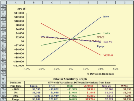
If we were comparing two projects, then the one with the steeper sensitivity lines would be riskier (other things held constant), because relatively small changes in the input variables would produce large changes in the NPV. Thus, sensitivity analysis provides useful insights into a project’s risk.9 Note, however, that even though NPV may be highly sensitive to certain variables, if those variables are not likely to change much from their expected values, then the project may not be very risky in spite of its high sensitivity. Also, if several of the inputs change at the same time, the combined effect on NPV can be much greater than sensitivity analysis suggests.
3. Scenario Analysis
- In the sensitivity analysis just described, we changed one variable at a time. However, it is useful to know what would happen to the project’s NPV if several of the inputs turn out to be better or worse than expected, and this is what we do in a scenario analysis. Also, scenario analysis allows us to assign probabilities to the base (or most likely) case, the best case, and the worst case; then we can find the expected value and standard deviation of the project’s NPV to get a better idea of the project’s risk.
- In a scenario analysis, we begin with the base-case scenario, which uses the most likely value for each input variable. We then ask marketing, engineering, and other operating managers to specify a worst-case scenario (low unit sales, low sales price, high variable costs, and so on) and a best-case scenario. Often, the best and worst cases are defined as having a 25% probability of occurring, with a 50% probability for the base-case conditions. Obviously, conditions could take on many more than three values, but such a scenario setup is useful to help get some idea of the project’s riskiness.
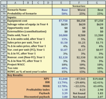
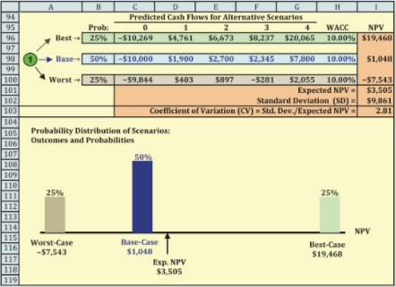
The project’s cash flows and performance measures under each scenario are calculated. The net cash flows for each scenario are shown in Figure 11-6, along with a probability distribution of the possible outcomes for NPV. If the project is highly successful, then a low initial investment, high sales price, high unit sales, and low production costs would combine to result in a very high NPV, $19,468. However, if things turn out badly, then the NPV would be a negative $7,543. This wide range of possibilities, and especially the large potential negative value, suggests that this is a risky project. If bad conditions materialize, the project will not bankrupt the company— this is just one project for a large company. Still, losing $7,543 (actually $7,543,000, as the units are thousands of dollars) would certainly hurt the company’s value and the reputation of the project’s manager.
If we multiply each scenario’s probability by the NPV for that scenario and then sum the products, we will have the project’s expected NPV of $3,505, as shown in Figure 11-6. Note that the expected NPV differs from the base-case NPV, which is the most likely outcome because it has a 50% probability. This is not an error—mathematically they are not equal.10 We also calculate the standard deviation of the expected NPV; it is $9,861. Dividing the standard deviation by the expected NPV yields the coefficient of variation, 2.81, which is a measure of stand-alone risk. The coefficient of variation measures the amount of risk per dollar of NPV, so the coefficient of variation can be helpful when comparing the risk of projects with different NPVs. GPC’s average project has a coeffi- cient of variation of about 1.2, so the 2.81 indicates that this project is riskier than most of GPC’s other typical projects.
GPC’s corporate WACC is 9%, so that rate should be used to find the NPV of an average-risk project. However, the water heater project is riskier than average, so a higher discount rate should be used to find its NPV. There is no way to determine the precisely correct discount rate—this is a judgment call. Management decided to evaluate the project using a 10% rate.
Note that the base-case results are the same in our sensitivity and scenario analyses, but in the scenario analysis the worst case is much worse than in the sensitivity analysis and the best case is much better. This is because in scenario analysis all of the variables are set at their best or worst levels, whereas in sensitivity analysis only one variable is adjusted and all the others are left at their base-case levels.
The project has a positive NPV, but its coefficient of variation (CV) is 2.81, which is more than double the 1.2 CV of an average project. With the higher risk, it is not clear if the project should be accepted or not. At this point, GPC’s CEO will ask the CFO to investigate the risk further by performing a simulation analysis.
4. Monte Carlo Simulation
- Monte Carlo simulation ties together sensitivities, probability distributions, and correlations among the input variables. It grew out of work in the Manhattan Project to build the first atomic bomb and was so named because it utilized the mathematics of casino gambling. Although Monte Carlo simulation is considerably more complex than scenario analysis, simulation software packages make the process manageable. Many of these packages can be used as add-ins to Excel and other spreadsheet programs.
- In a simulation analysis, a probability distribution is assigned to each input variable—sales in units, the sales price, the variable cost per unit, and so on. The computer begins by picking a random value for each variable from its probability distribution. Those values are then entered into the model, the project’s NPV is calculated, and the NPV is stored in the computer’s memory. This is called a trial. After completing the first trial, a second set of input values is selected from the input variables’ probability distributions, and a second NPV is calculated. This process is repeated many times. The NPVs from the trials can be charted on a histogram, which shows an estimate of the project’s outcomes. The average of the trials’ NPVs is interpreted as a measure of the project’s expected NPV, with the standard deviation (or the coefficient of variation) of the trials’ NPV as a measure of the project’s risk.
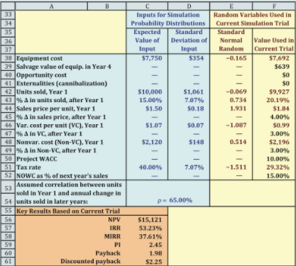
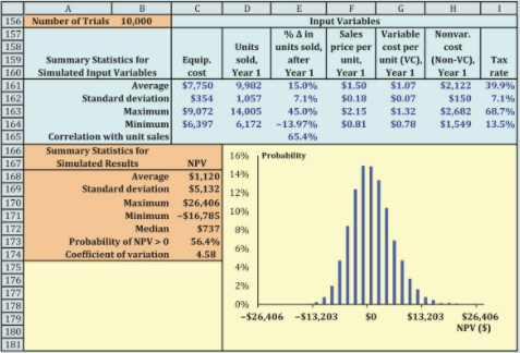
- Using this procedure, we conducted a simulation analysis of GPC’s solar water heater project. To compare apples and apples, we focused on the same six variables that were allowed to change in the previously conducted scenario analysis. We assumed that each variable can be represented by its own continuous normal distribution with means and standard deviations that are consistent with the base-case scenario. For example, we assumed that the units sold in Year 1 come from a normal distribution with a mean equal to the base-case value of 10,000. We used the probabilities and outcomes of the three scenarios from the previous Section to estimate the standard deviation. The standard deviation of units sold is 1,061, as calculated using the scenario values. We made similar assumptions for all variables. In addition, we assumed that the annual change in unit sales will be positively correlated with unit sales in the first year: If demand is higher than expected in the first year, it will continue to be higher than expected. In particular, we assume a correlation of 0.65 between units sold in the first year and growth in units sold in later years. For all other variables, we assumed zero correlation. The Figure below shows the inputs used in the simulation analysis.
- The Figure below also shows the current set of random variables that were drawn from the distributions at the time we created the figure for the textbook—you will see different values for the key results when you look at the Excel model because the values are updated every time the file is opened. We used a two-step procedure to create the random variables for the inputs. First, we used Excel’s functions to generate standard normal random variables with a mean of 0 and a standard deviation of 1; these are shown in Cells E38: E51.13 To create the random values for the inputs used in the analysis, we multiplied a random standard normal variable by the standard deviation and added the expected value. For example, Excel drew the value −0.07 for first-year unit sales (Cell E42) from a standard normal distribution. We calculated the value for first-year unit sales to use in the current trial as 10,000 + 1,061(−0.07) = 9,927, which is shown in Cell F42.
- We used the inputs in Cells F38:F52 to generate cash flows and to calculate perfor- mance measures for the project (the calculations are in the Tool Kit). For the trial reported in Figure 11-7, the NPV is $15,121. We used a Data Table in the Tool Kit to generate additional trials. For each trial, the Data Table saved the value of the input variables and the value of the trial’s NPV. Figure 11-8 presents selected results from the simulation for 10,000 trials.
- After running a simulation, the first thing we do is verify that the results are consistent with our assumptions. The resulting sample mean and standard deviation of units sold in the first year are 9,982 and 1,057, which are virtually identical to our assumptions in the Figure below. The same is true for all the other inputs, so we can be reasonably confident that the simulation is doing what we are asking. Figure 11-8 also reports summary statistics for the project’s NPV. The mean is $1,120, which suggests that the project should be accepted. However, the range of outcomes is quite large, from a loss of $16,785 to a gain of $26,406, so the project is clearly risky. The standard deviation of $5,132 indicates that losses could easily occur, which is consistent with this wide range of possible outcomes.15 Figure 11-8 also reports a median NPV of $737, which means that half the time the project will have an NPV of less than $737. In fact, there is only 56.4% probability that the project will have a positive NPV.
A picture is worth a thousand words, and the Figure below shows the probability distribution of the outcomes. Note that the distribution of outcomes is slightly skewed to the right. As the figure shows, the potential downside losses are not as large as the potential upside gains. Our conclusion is that this is a very risky project, as indicated by the coefficient of variation, but it does have a positive expected NPV and the potential to be a “home run.”
If the company decides to go ahead with the project, senior management should also identify possible contingency plans for responding to changes in market conditions. Senior managers always should consider qualitative factors in addition to the quantitative project analysis.
Last modified: Tuesday, August 14, 2018, 8:51 AM