Reading: Lesson 6 - Project Risk Conclusions
9.6.A - Project Risk Conclusions
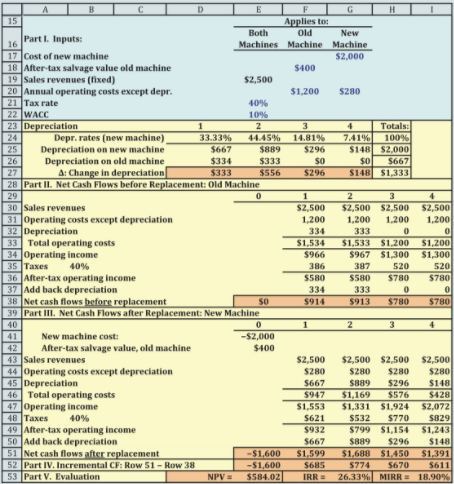
1. Replacement Analysis
- In the previous sections we assumed that the solar water heater project was an entirely new project, so all of its cash flows were incremental—they would occur if and only if the project were accepted. However, for replacement projects we must find the cash flow differentials between the new and old projects, and these differentials are the incremental cash flows that we must analyze.
- In some instances, replacements add capacity as well as lower operating costs. In this case, sales revenues in Part III would be increased, and if that leads to a need for more working capital, then this would be shown as a Time 0 expenditure along with a recovery at the end of the project’s life. These changes would, of course, be reflected in the incremental cash flows on Row 52.
2. Real Options
- According to traditional capital budgeting theory, a project’s NPV is the present value of its expected future cash flows discounted at a rate that reflects the riskiness of those cash flows. Note, however, that this says nothing about actions taken after the project has been accepted and placed in operation that might lead to an increase in the cash flows. In other words, traditional capital budgeting theory assumes that a project is like a roulette wheel. A gambler can choose whether to spin the wheel, but once the wheel has been spun, nothing can be done to influence the outcome. Once the game begins, the outcome depends purely on chance, and no skill is involved.
- Capital budgeting decisions have more in common with poker than roulette because (1) chance plays a continuing role throughout the life of the project, but (2) managers can respond to changing market conditions and to competitors’ actions. Opportunities to respond to changing circumstances are called managerial options (because they give managers a chance to influence the outcome of a project), strategic options (because they are often associated with large, strategic projects rather than routine maintenance projects), and embedded options (because they are a part of the project). Finally, they are called real options to differentiate them from financial options because they involve real, rather than financial, assets. The following sections describe projects with several types of real options.
- Conventional NPV analysis implicitly assumes that projects either will be accepted or rejected, which implies they will be undertaken now or never. In practice, however, companies sometimes have a third choice—delay the decision until later, when more information is available. Such investment timing options can dramatically affect a project’s estimated profitability and risk, as we saw in our example of GPC’s solar water heater project.
- Keep in mind, though, that the option to delay is valuable only if it more than offsets any harm that might result from delaying. For example, while one company delays, some other company might establish a loyal customer base that makes it difficult for the first company to enter the market later. The option to delay is usually most valuable to firms with proprietary technology, patents, licenses, or other barriers to entry, because these factors lessen the threat of competition. The option to delay is valuable when market demand is uncertain, but it is also valuable during periods of volatile interest rates, because the ability to wait can allow firms to delay raising capital for a project until interest rates are lower.
- A growth option allows a company to increase its capacity if market conditions are better than expected. There are several types of growth options. One lets a company increase the capacity of an existing product line. A “peaking unit” power plant illustrates this type of growth option. Such units have high variable costs and are used to produce additional power only if demand, thus prices, are high.
- The second type of growth option allows a company to expand into new geographic markets. Many companies are investing in China, Eastern Europe, and Russia even though standard NPV analysis produces negative NPVs. However, if these developing markets really take off, the option to open more facilities could be quite valuable.
- The third type of growth option is the opportunity to add new products, including complementary products and successive “generations” of the original product. Auto companies are losing money on their first electric autos, but the manufacturing skills and consumer recognition those cars will provide should help turn subsequent generations of electric autos into moneymakers.
- Consider the value of an abandonment option. Standard DCF analysis assumes that a project’s assets will be used over a specified economic life. But even though some projects must be operated over their full economic life—in spite of deteriorating market conditions and hence lower than expected cash flows—other projects can be abandoned. Smart managers negotiate the right to abandon if a project turns out to be unsuccessful as a condition for undertaking the project.
- Note, too, that some projects can be structured so that they provide the option to reduce capacity or temporarily suspend operations. Such options are common in the natural resources industry, including mining, oil, and timber, and they should be reflected in the analysis when NPVs are being estimated.
- Many projects offer flexibility options that permit the firm to alter operations depending on how conditions change during the life of the project. Typically, either inputs or outputs (or both) can be changed. BMW’s Spartanburg, South Carolina, auto assembly plant provides a good example of output flexibility. BMW needed the plant to produce sports coupes. If it built the plant configured to produce only these vehicles, the construction cost would be minimized. However, the company thought that later on it might want to switch production to some other vehicle type, and that would be difficult if the plant were designed just for coupes. Therefore, BMW decided to spend additional funds to construct a more flexible plant: one that could produce different types of vehicles should demand patterns shift. Sure enough, things did change. Demand for coupes dropped a bit and demand for sport-utility vehicles soared. But BMW was ready, and the Spartanburg plant began to produce hot-selling SUVs. The plant’s cash flows were much higher than they would have been without the flexibility option that BMW “bought” by paying more to build a more flexible plant.
- Electric power plants provide an example of input flexibility. Utilities can build plants that generate electricity by burning coal, oil, or natural gas. The prices of those fuels change over time in response to events in the Middle East, changing environmental policies, and weather conditions. Some years ago, virtually all power plants were designed to burn just one type of fuel, because this resulted in the lowest construction costs. However, as fuel cost volatility increased, power companies began to build higher-cost but more flexible plants, especially ones that could switch from oil to gas and back again depending on relative fuel prices.
- A full treatment of real option valuation is beyond the scope of this chapter, but there are some things we can say. First, if a project has an embedded real option, then management should at least recognize and articulate its existence. Second, we know that a financial option is more valuable if it has a long time until maturity or if the underlying asset is very risky. If either of these characteristics applies to a project’s real option, then management should know that its value is probably relatively high. Third, management might be able to model the real option along the lines of a decision tree, as we illustrate in the following section.
3. Phased Decisions and Decision Trees
- GPC’s analysis of the solar water heater project thus far has assumed that the project cannot be abandoned once it goes into operation, even if the worst-case situation arises. However, GPC is considering the possibility of terminating (abandoning) the project at Year 2 if the demand is low. The net after-tax cash flow from salvage, legal fees, liquidation of working capital, and all other termination costs and revenues is $5,000. Using these assumptions, the GPC ran a new scenario analysis; the results are shown in the Figure below, which is a simple decision tree.
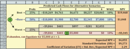
Here we assume that, if the worst case materializes, then this will be recognized after the low Year-1 cash flow and GPC will abandon the project. Rather than continue realizing low cash flows in Years 2, 3, and 4, the company will shut down the operation and liquidate the project for $5,000 at t = 2. Now the expected NPV rises from $3,505 to $4,055 and the CV declines from 2.81 to 2.29. So, securing the right to abandon the project if things don’t work out raised the project’s expected return and lowered its risk. This will give you an approximate value, but keep in mind that you may not have a good estimate of the appropriate discount rate because the real option changes the risk, and hence the required return, of the project.
After the management team thought about the decision-tree approach, other ideas for improving the project emerged. The marketing manager stated that he could undertake a study that would give the firm a better idea of demand for the product. If the marketing study found favorable responses to the product, the design engineer stated that she could build a prototype solar water heater to gauge consumer reactions to the actual product. After assessing consumer reactions, the company could either go ahead with the project or abandon it. This type of evaluation process is called a staged decision tree and is shown in the Figure below.
Decision trees such as the one in the Figure below often are used to analyze multistage, or sequential, decisions. Each circle represents a decision point, also known as a decision node. The dollar value to the left of each decision node represents the net cash flow at that point, and the cash flows shown under t = 3, 4, 5, and 6 represent the cash inflows if the project is pushed on to completion. Each diagonal line leads to a branch of the decision tree, and each branch has an estimated probability. For example, if the firm decides to “go” with the project at Decision Point 1, then it will spend $100,000 on the marketing study. Management estimates that there is a 0.8 probability that the study will produce positive results, leading to the decision to make an additional investment and thus move on to Decision Point 2, and a 0.2 probability that the marketing study will produce negative results, indicating that the project should be canceled after Stage 1. If the project is canceled, the cost to the company will be the $100,000 spent on the initial marketing study.
If the marketing study yields positive results, then the firm will spend $500,000 on the prototype water heater module at Decision Point 2. Management estimates (even before making the initial $100,000 investment) that there is a 45% probability of the pilot project yielding good results, a 40% probability of average results, and a 15% probability of bad results. If the prototype works well, then the firm will spend several millions more at Decision Point 3 to build a production plant, buy the necessary inventory, and commence operations. The operating cash flows over the project’s 4-year life will be good, average, or bad, and these cash flows are shown under Years 3 through 6.
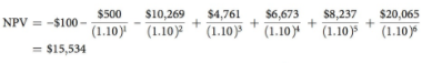
The column of joint probabilities in the Figure above gives the probability of occurrence of each branch—and hence of each NPV. Each joint probability is obtained by multiplying together all the probabilities on that particular branch. For example, the probability that the company will, if Stage 1 is undertaken, move through Stages 2 and 3, and that a strong demand will produce the indicated cash flows, is (0.8)(0.45) = 0.36 = 36.0%. There is a 32% probability of average results, a 12% probability of building the plant and then getting bad results, and a 20% probability of getting bad initial results and stopping after the marketing study. The NPV of the top (most favorable) branch as shown in Column J is $15,534, calculated as follows:
The last column in the Figure above gives the product of the NPV for each branch times the joint probability of that branch’s occurring, and the sum of these products is the project’s expected NPV. Based on the expectations used to create the Figure above and a cost of capital of 10%, the project’s expected NPV is $5,606, or $5.606 million.19 In addition, the CV declines from 2.81 to 1.33, and the maximum anticipated loss is a manageable −$555,000. At this point, the solar water heater project looked good, and GPC’s management decided to accept it.
As this example shows, decision-tree analysis requires managers to articulate explicitly the types of risk a project faces and to develop responses to potential scenarios. Note also that our example could be extended to cover many other types of decisions and could even be incorporated into a simulation analysis. All in all, decision-tree analysis is a valuable tool for analyzing project risks.
Last modified: Tuesday, August 14, 2018, 8:51 AM