Reading: Lesson 1 - Financial Planning
10.1.A - Financial Planning & Forecasting Operations
1. Financial Planning
- A vital step in financial planning is to forecast financial statements, which are called projected financial statements or pro forma financial statements. Managers use projected financial statements in four ways: (1) By looking at projected statements, they can assess whether the firm’s anticipated performance is in line with the firm’s own general targets and with investors’ expectations. (2) Pro forma statements can be used to estimate the effect of proposed operating changes, enabling managers to conduct “what if” analyses. (3) Managers use pro forma statements to anticipate the firm’s future financing needs. (4) Managers forecast free cash flows under different operating plans, forecast their capital requirements, and then choose the plan that maximizes shareholder value. Security analysts make the same types of projections, forecasting future earnings, cash flows, and stock prices.
- The two most important components of financial planning are the operating plan and the financial plan.
- An operating plan provides detailed implementation guidance for a firm’s operations, including the firm’s choice of market segments, product lines, sales and marketing strategies, production processes, and logistics. An operating plan can be developed for any time horizon, but most companies use a 5-year horizon, with the plan being quite detailed for the first year but less and less specific for each succeeding year. The plan explains who is responsible for each particular function and when specific tasks are to be accomplished.
- An important part of the operating plan is the forecast of sales, production costs, inventories, and other operating items. In fact, this part of the operating plan actually is a forecast of the company’s expected free cash flow. Free cash flow is the primary source of a company’s value. Using what-if analysis, managers can analyze different operating plans to estimate their impact on value. In addition, managers can apply sensitivity analysis, scenario analysis, and simulation to estimate the risk of different operating plans, which is an important part of risk management.
- By definition, a company’s operating assets can grow only by the purchase of additional assets. Therefore, a growing company must continually obtain cash to purchase new assets. Some of this cash might be generated internally by its operations, but some might have to come externally from shareholders or debtholders. This is the essence of financial planning—forecasting the additional sources of financing required to fund the operating plan.
- There is a strong connection between financial planning and free cash flow. A company’s operations generate the free cash flow, but the financial plan determines how the company will use the free cash flow. Recall from Unit 1 that free cash flow can be used in five ways: (1) pay dividends, (2) repurchase stock, (3) pay the net after-tax interest on debt, (4) repay debt, or (5) purchase financial assets such as marketable securities. A company’s financial plan must use free cash flow differently if FCF is negative than if FCF is positive.
- If free cash flow is positive, the financial plan must identify how much FCF to allocate among its investors (shareholders or debtholders) and how much to put aside for future needs by purchasing marketable securities. If free cash flow is negative, either because the company is growing rapidly (which requires large investments in operating capital) or because the company has low NOPAT, then the total uses of free cash flow must also be negative. For example, instead of repurchasing stock, the company might have to issue stock; instead of repaying debt, the company might have to issue debt.
- Therefore, the financial plan must incorporate (1) the company’s dividend policy, which determines the targeted size and method of cash distributions to shareholders, and (2) the capital structure, which determines the targeted mix of debt and equity used to finance the firm, which in turn determines the relative mix of distributions to shareholders and payments to debtholders.
2. Financial Planning Example
- As we described in Sections 2 and 3, MicroDrive’s operating performance and stock price have declined in recent years. As a result, MicroDrive’s board recently installed a new management team: A new CEO, CFO, marketing manager, sales manager, inventory manager, and credit manager—only the production manager was retained. The new team met for a 3-day retreat with the goal of developing a plan to improve the company’s performance.
- One of the first steps was to develop forecasts based on the status quo to give the management team a better idea of where the company is now and where it will be if they don’t make changes. The new CFO began by developing an Excel model to forecast the operating plan and the financial plan.
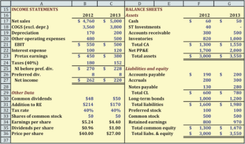
- The CFO’s first step was to examine the current and recent historical data. The Figure below shows MicroDrive’s most recent financial statements and selected additional data.
The CFO’s second step was to choose a forecasting framework. Many companies, including MicroDrive, forecast their entire financial statements as part of the planning process. This approach is called forecasted financial statements (FFS) method of financial planning.
The Figure below shows the inputs MicroDrive uses to forecast different scenarios for its operating plan and financial plan. The inputs are for the Status Quo scenario, which assumes most of MicroDrive’s operating activities and financial policies remain unchanged. The figure shows actual values for industry peers (the silver section), actual values for MicroDrive’s past two years, and forecasted values for MicroDrive’s 5-year forecast. The blue section shows inputs for the first year and inputs for any subsequent years that differ from the previous year. Section 1 shows the ratios required to project the items required for an operating plan, Section 2 shows the inputs related to the capital structure, Section 3 shows the costs of the capital components, and Section 4 shows the target dividend policy. We will describe each of these sections as they are applied to the forecast, beginning with the forecast of operations.
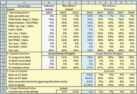
The first row in Section 1 of the Figure above shows the forecast of the sales growth rate. After discussions with teams from marketing, sales, product development, and production, MicroDrive’s CFO chose a growth rate of 10% for the next year. Keep in mind that this is just a preliminary estimate and that it is easy to make changes in the Excel model (after doing the hard work to build the model!). Notice that MicroDrive is forecasting sales growth to decline and level off by the end of the forecast. Recall from Section 7 that the growth rate for a company’s sales and free cash flows must level off at some future date in order to apply the constant growth model at the forecast horizon. Had MicroDrive’s managers projected non-constant growth for more than five years, the Figure above would need to be extended until growth does level out.
Other than sales growth, MicroDrive’s managers assumed that the operating ratios for 2014 would remain constant for the entire forecast period. However, it would be quite easy for them to input changes in the future ratios, with one caveat. The operating ratios must level off by the end of the forecast period, or else the free cash flows will not be growing at a constant rate by the end of the forecast period even if sales are growing at a constant rate.
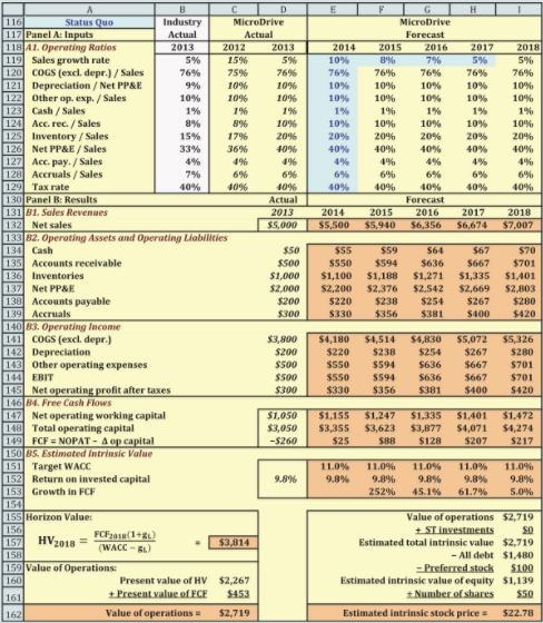
Section B1 of the Figure below shows the forecast of net sales based on the previous year’s sales and the forecasted growth rate in sales. For example, the forecast of net sales for 2014 is (1 + 0.10)($5,000) = $5,500.
Section B2 of the Figure below shows the forecast of operating assets. As noted earlier, MicroDrive’s assets must increase if sales are to increase, and some types of assets grow proportionately to sales, including cash.
MicroDrive writes and deposits checks every day. Because its managers don’t know exactly when all of the checks will clear, they can’t predict exactly what the balance in their checking accounts will be on any given day. Therefore, they must maintain a balance of cash and cash equivalents (such as very short-term marketable securities) to avoid overdrawing their accounts. We discuss the issue of cash management in Chapter 16, but MicroDrive’s CFO assumed that the cash required to support MicroDrive’s operations is proportional to its sales. For example, the forecasted cash in 2014 is 1%(2014 sales) = 1%($5,500) = $55. The CFO applied the same process to project cash in subsequent years.
Unless a company changes its credit policy or has a change in its customer base, accounts receivable should be proportional to sales. The CFO assumed that the credit policy and customers’ paying patterns would remain constant and so projected accounts receivable as 10%($5,500) = $550.
As sales increase, firms generally must carry more inventories. The CFO assumed here that inventory would be proportional to sales. (Chapter 16 will discuss inventory management in detail). The projected inventory is 20%($5,500) = $1,100.
It might be reasonable to assume that cash, accounts receivable, and inventories will be proportional to sales, but will the amount of net property, plant, and equipment go up and down as sales go up and down? The correct answer could be either yes or no. When companies acquire PP&E, they often install more capacity than they currently need due to economies of scale in building capacity. Moreover, even if a plant is operating at its maximum-rated capacity, most companies can produce additional units by reducing downtime for scheduled maintenance, by running machinery at a higher than optimal speed, or by adding a second or third shift. Therefore, at least in the short run, sales and net PP&E may not have a close relationship.
Section B2 of the Figure above shows the forecast of operating liabilities. Some types of liabilities grow proportionately to sales; these are called spontaneous liabilities, as we explain next. As sales increase, so will purchases of raw materials, and those additional purchases will spontaneously lead to a higher level of accounts payable. MicroDrive’s forecast of accounts payable in 2014 is 4%($5,500) = $220. Higher sales require more labor, and higher sales normally result in higher taxable income and thus taxes. Therefore, accrued wages and taxes both increase as sales increase. The projection of accruals is 6%($5,500) = $330.
For most companies, the cost of goods sold (COGS) is highly correlated with sales, and MicroDrive is no exception. MicroDrive’s forecast of COGS for 2014 is 76%($5,500) = $4,180. Because depreciation depends on an asset’s depreciable basis, as described in Chapter 11, it is more reasonable to forecast depreciation as a percent of net plant and equipment rather than of sales. MicroDrive’s projection of depreciation in 2014 is 10%(2014 Net PP&E) = 10%($2,200) = $220. MicroDrive’s other operating expenses include items such as salaries of executives, insurance fees, and marketing costs. These items tend to be related to a company’s size, which is related to sales. MicroDrive’s projection is 10%($5,500) = $550. Subtracting the COGS, depreciation, and other operating expenses from net sales gives the earnings before interest and taxes (EBIT). Recall from Chapter 2 that the net operating profit after taxes (NOPAT) is defined as EBIT(1 − T), where T is the tax rate.
Section B4 calculates free cash flow (FCF) using the process described in Section 2. The first row in Section B4 begins with a calculation of net operating capital (NOWC), which is defined as operating current assets minus operating current liabilities. Operating current assets is the sum of cash, accounts receivable, and inventories; operating current liabilities is the sum or accounts payable and accruals. The second row shows the forecast of total operating capital, which is NOWC plus net PP&E. All of the items required for these calculations were previously forecast in Section B2.
3. Estimated Intrinsic Value
- Section B5 begins with the estimated target WACC, calculated using the inputs from Sections 2 and 3 of the Figure above. These values are the same ones used in earlier to estimate MicroDrive’s weighted average cost of capital, with the exception of the cost of preferred stock. To simplify the forecast of preferred dividends when projecting the income statement, MicroDrive’s CFO decided to ignore flotation costs because they have a negligible impact on the WACC.
- The weighted average cost of capital is calculated based on the target capital structure. MicroDrive’s CFO decided to use the target capital structure for all scenarios, but to modify the projections later if the board decides to change the capital structure.
- The second row in Section B5 of the Figure above reports return on invested capital (ROIC) for easy comparison to the WACC. The third row shows the growth rate in FCF. Notice that the growth rate is very high in the early years of the forecast but then levels out at the sustainable growth rate of sales, 5%. Had it not done so, the forecast period would need to be extended until the growth in FCF became constant.
- Using the estimated FCF, WACC, and long-term constant growth rate in FCF, Section B5 shows the calculation of the value of operations using the constant growth horizon value formula. To find the value of operations, it is necessary to find the present value of the horizon value and the present value of the forecasted free cash flows, and then sum them, as shown at the lower-left corner of the figure.
- The panel on the lower right of Section B5 estimates the intrinsic stock price using the approach. For the Status Quo forecast, the estimated intrinsic value is $22.78. This estimate is about 16% lower than the price of $27 observed on December 31, 2013. What can account for this difference? First, keep in mind that MicroDrive’s standard deviation of stock returns is about 49%. This high standard deviation makes the 16% difference between the estimated and actual stock price look pretty small. It could well be that the estimated intrinsic value would have been exactly equal to the actual stock price on a day during the week before or after December 31, 2013. Second, it could be that investors (who determine the price through their buying and selling activities) expect MicroDrive’s performance in the future to be better than the Status Quo scenario.
Last modified: Tuesday, August 14, 2018, 8:52 AM