Reading: Lesson 3 - Capital Structure Theory
12.3.A - Capital Structure Theory
1. Modigliani and Miller: No Taxes
- In the previous section, we showed how capital structure choices affect a firm’s ROE and its risk. For a number of reasons, we would expect capital structures to vary considerably across industries. For example, pharmaceutical companies generally have very different capital structures than airline companies. Moreover, capital structures vary among firms within a given industry. What factors explain these differences? In an attempt to answer this question, academics and practitioners have developed a number of theories, and the theories have been subjected to many empirical tests. The following sections examine several of these theories.
- Modern capital structure theory began in 1958, when Professors Franco Modigliani and Merton Miller (hereafter MM) published what has been called the most influential finance article ever written. MM’s study was based on some strong assumptions, which included the following:
1. There are no brokerage costs.
2. There are no taxes.
3. There are no bankruptcy costs.
4. Investors can borrow at the same rate as corporations.
5. All investors have the same information as management about the firm’s future investment opportunities.
6. EBIT is not affected by the use of debt. - Modigliani and Miller imagined two hypothetical portfolios. The first contains all the equity of an unlevered firm, so the portfolio’s value is VU, the value of an unlevered firm. Because the firm has no growth (which means it does not need to invest in any new net assets) and because it pays no taxes, the firm can pay out all of its EBIT in the form of dividends. Therefore, the cash flow from owning this first portfolio is equal to EBIT.
- Now consider a second firm that is identical to the unlevered firm except that it is partially financed with debt. The second portfolio contains all of the levered firm’s stock (SL) and debt (D), so the portfolio’s value is VL, the total value of the levered firm. If the interest rate is rd, then the levered firm pays out interest in the amount rdD. Because the firm is not growing and pays no taxes, it can pay out dividends in the amount EBIT − rdD. If you owned all of the firm’s debt and equity, your cash flow would be equal to the sum of the interest and dividends: rdD + (EBIT − rdD) = EBIT. Therefore, the cash flow from owning this second portfolio is equal to EBIT.
- Notice that the cash flow of each portfolio is equal to EBIT. Thus, MM concluded that two portfolios producing the same cash flows must have the same value:

Recall that the WACC is a combination of the cost of debt and the relatively higher cost of equity, rs. As leverage increases, more weight is given to low-cost debt but equity becomes riskier, which drives up rs. Under MM’s assumptions, rs increases by exactly enough to keep the WACC constant. Put another way: If MM’s assumptions are correct, then it doesn’t matter how a firm finances its operations and so capital structure decisions are irrelevant.
Even though some of their assumptions are obviously unrealistic, MM’s irrelevance result is extremely important. By indicating the conditions under which capital structure is irrelevant, MM also provided us with clues about what is required for capital structure to be relevant and hence to affect a firm’s value. The work of MM marked the beginning of modern capital structure research, and subsequent research has focused on relaxing the MM assumptions in order to develop a more realistic theory of capital structure.
Modigliani and Miller’s thought process was just as important as their conclusion. It seems simple now, but their idea that two portfolios with identical cash flows must also have identical values changed the entire financial world because it led to the development of options and derivatives. It is no surprise that Modigliani and Miller received Nobel awards for their work.
2. Modigliani and Miller II: The Effect of Corporate Taxes
- In 1963, MM published a follow-up paper in which they relaxed the assumption that there are no corporate taxes. The Tax Code allows corporations to deduct interest payments as an expense, but dividend payments to stockholders are not deductible. The differential treatment encourages corporations to use debt in their capital structures. This means that interest payments reduce the taxes a corporation pays, and if a corporation pays less to the government, then more of its cash flow is available for investors. In other words, the tax deductibility of the interest payments shields the firm’s pre-tax income.
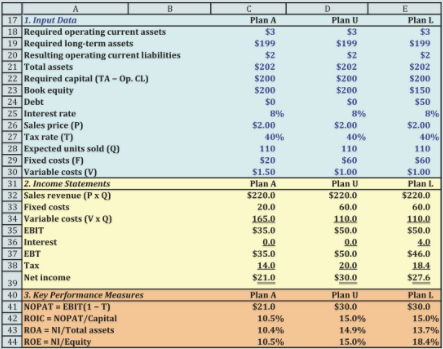
- To illustrate, look at the Figure below and see that Plan U (with no debt) pays taxes of $20, but Plan L (with leverage) pays taxes of only $18.40. What happens to the difference of $1.60 = $20 − $18.40? Notice that Plan U has $30 of net income for shareholders, but Plan U has $4 of interest for debtholders and $27.60 of net income for shareholders for a combined total of $31.60, which is exactly $1.60 more than Plan U. With more cash flows available for investors, a levered firm’s total value should be greater than that of an unlevered firm, and this is what MM showed.
As in their earlier paper, MM introduced a second important way of looking at the effect of capital structure: The value of a levered firm is the value of an otherwise identical unlevered firm plus the value of any “side effects.” While others have expanded on this idea by considering other side effects, MM focused on the tax shield:

Under their assumptions, they showed that the present value of the tax shield is equal to the corporate tax rate, T, multiplied by the amount of debt, D:

With a tax rate of about 40%, this implies that every dollar of debt adds about 40 cents of value to the firm, and this leads to the conclusion that the optimal capital structure is virtually 100% debt. MM also showed that the cost of equity, rs, increases as leverage increases but that it doesn’t increase quite as fast as it would if there were no taxes. As a result, under MM with corporate taxes the WACC falls as debt is added.
3. Miller: The Effect of Corporate and Personal Taxes
- Merton Miller (this time without Modigliani) later brought in the effects of personal taxes. The income from bonds is generally interest, which is taxed as personal income at rates (Td) going up to 35%, while income from stocks generally comes partly from dividends and partly from capital gains. Long-term capital gains are taxed at a rate of 15%, and this tax is deferred until the stock is sold and the gain realized. If stock is held until the owner dies, no capital gains tax whatsoever must be paid. So, on average, returns on stocks are taxed at lower effective rates (Ts) than returns on debt.
- Because of the tax situation, Miller argued that investors are willing to accept relatively low before-tax returns on stock relative to the before-tax returns on bonds. (The situation here is similar to that with tax-exempt municipal bonds and preferred stocks held by corporate investors.) For example, an investor might require a return of 10% on Strasburg’s bonds, and if stock income were taxed at the same rate as bond income, the required rate of return on Strasburg’s stock might be 16% because of the stock’s greater risk. However, in view of the favorable treatment of income on the stock, investors might be willing to accept a before-tax return of only 14% on the stock.
- Thus, as Miller pointed out, (1) the deductibility of interest favors the use of debt financing, but (2) the more favorable tax treatment of income from stock lowers the required rate of return on stock and thus favors the use of equity financing. Miller showed that the net impact of corporate and personal taxes is given by this equation:

Here Tc is the corporate tax rate, Ts is the personal tax rate on income from stocks, and Td is the tax rate on income from debt. Miller argued that the marginal tax rates on stock and debt balance out in such a way that the bracketed term in the Equation below is zero and so VL = VU, but most observers believe there is still a tax advantage to debt if reasonable values of tax rates are assumed. For example, if the marginal corporate tax rate is 40%, the marginal rate on debt is 30%, and the marginal rate on stock is 12%, then the advantage of debt financing is

Thus it appears that the presence of personal taxes reduces but does not completely eliminate the advantage of debt financing.
4. Trade-Off Theory
- The results of Modigliani and Miller also depend on the assumption that there are no bankruptcy costs. However, bankruptcy can be quite costly. Firms in bankruptcy have very high legal and accounting expenses, and they also have a hard time retaining customers, suppliers, and employees. Moreover, bankruptcy often forces a firm to liquidate or sell assets for less than they would be worth if the firm were to continue operating. For example, if a steel manufacturer goes out of business it might be hard to find buyers for the company’s blast furnaces. Such assets are often illiquid because they are configured to a company’s individual needs and also because they are difficult to disassemble and move.
- Note, too, that the threat of bankruptcy, not just bankruptcy per se, causes many of these same problems. Key employees jump ship, suppliers refuse to grant credit, customers seek more stable suppliers, and lenders demand higher interest rates and impose more restrictive loan covenants if potential bankruptcy looms. Therefore, even the threat of bankruptcy can cause free cash flows to fall, causing further declines in a company’s value.
- Bankruptcy-related problems are most likely to arise when a firm includes a great deal of debt in its capital structure. Therefore, bankruptcy costs discourage firms from pushing their use of debt to excessive levels.
- Bankruptcy-related costs have two components: (1) the probability of financial distress and (2) the costs that would be incurred if financial distress does occur. Firms whose earnings are more volatile, all else equal, face a greater chance of bankruptcy and should therefore use less debt than more stable firms. This is consistent with our earlier point that firms with high operating leverage, and thus greater business risk, should limit their use of financial leverage. Likewise, firms that would face high costs in the event of financial distress should rely less heavily on debt. For example, firms whose assets are illiquid and thus would have to be sold at “fire sale” prices should limit their use of debt financing.
- The preceding arguments led to the development of what is called the trade-off theory of leverage, in which firms trade off the benefits of debt financing (favorable corporate tax treatment) against higher interest rates and bankruptcy costs. In essence, the trade-off theory says that the value of a levered firm is equal to the value of an unlevered firm plus the value of any side effects, which include the tax shield and the expected costs due to financial distress. A summary of the trade-off theory is expressed graphically in the Figure below, and a list of observations about the figure follows here.
1. Under the assumptions of the MM model with corporate taxes, a firm’s value increases linearly for every dollar of debt. The line labeled “MM Result Incorporating the Effects of Corporate Taxation” in the Figure below expresses the relationship between value and debt under those assumptions.
2. There is some threshold level of debt, labeled D1 in the Figure below, below which the probability of bankruptcy is so low as to be immaterial. Beyond D1, however, expected bankruptcy-related costs become increasingly important, and they reduce the tax benefits of debt at an increasing rate. In the range from D1 to D2, expected bankruptcy-related costs reduce but do not completely offset the tax benefits of debt, so the stock price rises (but at a decreasing rate) as the debt ratio increases. However, beyond D2, expected bankruptcy-related costs exceed the tax benefits, so from this point on increasing the debt ratio lowers the value of the stock. Therefore, D2 is the optimal capital structure. Of course, D1 and D2 vary from firm to firm, depending on their business risks and bankruptcy costs.
3. Although theoretical and empirical work confirms the general shape of the curve in the Figure below, this graph must be taken as an approximation and not as a precisely defined function.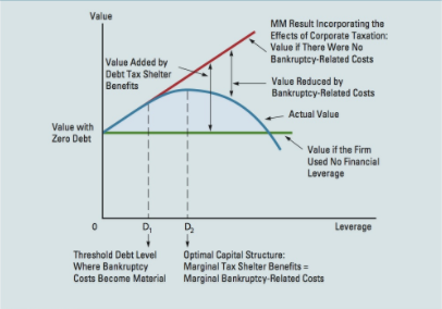
5. Signaling Theory
- MM assumed that investors have the same information about a firm’s prospects as its managers—this is called symmetric information. However, managers in fact often have better information than outside investors. This is called asymmetric information, and it has an important effect on the optimal capital structure. To see why, consider two situations, one in which the company’s managers know that its prospects are extremely positive (Firm P) and one in which the managers know that the future looks negative (Firm N).
- Suppose, for example, that Firm P’s R&D labs have just discovered a cure for the common cold. Firm P can’t provide investors with any details about the product because that might give competitors an advantage. But if they don’t provide details, then investors will underestimate the value of the discovery. Given the inability to provide accurate, verifiable information to the market, how should Firm P’s management raise the needed capital?
- Suppose Firm P issues stock. When profits from the new product start flowing in, the price of the stock would rise sharply and the purchasers of the new stock would make a bonanza. The current stockholders (including the managers) would also do well, but not as well as they would have done if the company had not sold stock before the price increased, because then they would not have had to share the benefits of the new product with the new stockholders. Therefore, we should expect a firm with very positive prospects to avoid selling stock and instead to raise required new capital by other means, including debt usage beyond the normal target capital structure.
- Now let’s consider Firm N. Suppose its managers have information that new orders are off sharply because a competitor has installed new technology that has improved its products’ quality. Firm N must upgrade its own facilities, at a high cost, just to maintain its current sales. As a result, its return on investment will fall (but not by as much as if it took no action, which would lead to a 100% loss through bankruptcy). How should Firm N raise the needed capital? Here the situation is just the reverse of that facing Firm P, which did not want to sell stock so as to avoid having to share the benefits of future developments. A firm with negative prospects would want to sell stock, which would mean bringing in new investors to share the losses. The conclusion from all this is that firms with extremely bright prospects prefer not to finance through new stock offerings, whereas firms with poor prospects like to finance with outside equity. How should you, as an investor, react to this conclusion? You ought to say: “If I see that a company plans to issue new stock, this should worry me because I know that management would not want to issue stock if future prospects looked good. However, management would want to issue stock if things looked bad. Therefore, I should lower my estimate of the firm’s value, other things held constant, if it plans to issue new stock.”
- If you gave this answer, then your views are consistent with those of sophisticated portfolio managers. In a nutshell: The announcement of a stock offering is generally taken as a signal that the firm’s prospects as seen by its own management are not good; conversely, a debt offering is taken as a positive signal. Notice that Firm N’s managers cannot make a false signal to investors by mimicking Firm P and issuing debt. With its unfavorable future prospects, issuing debt could soon force Firm N into bankruptcy. Given the resulting damage to the personal wealth and reputations of N’s managers, they cannot afford to mimic Firm P. All of this suggests that when a firm announces a new stock offering, more often than not the price of its stock will decline. Empirical studies have shown that this is indeed true.
6. Market Timing Theory
- If markets are efficient, then security prices should reflect all available information; hence they are neither underpriced nor overpriced (except during the time it takes prices to move to a new equilibrium caused by the release of new information). The market timing theory states that managers don’t believe this and supposes instead that stock prices and interest rates are sometimes either too low or too high relative to their true fundamental values. In particular, the theory suggests that managers issue equity when they believe stock market prices are abnormally high and issue debt when they believe interest rates are abnormally low. In other words, they try to time the market. Notice that this differs from signaling theory because no asymmetric information is involved. These managers aren’t basing their beliefs on insider information, just on a different opinion than the market consensus.
Last modified: Tuesday, August 14, 2018, 8:55 AM